This PDF is a selection from an out-of-print volume from the National Bureau
of Economic Research
Volume Title: Reducing Inflation: Motivation and Strategy
Volume Author/Editor: Christina D. Romer and David H. Romer, Editors
Volume Publisher: University of Chicago Press
Volume ISBN: 0-226-72484-0
Volume URL: http://www.nber.org/books/rome97-1
Conference Date: January 11-13, 1996
Publication Date: January 1997
Chapter Title: How the Bundesbank Conducts Monetary Policy
Chapter Author: Richard H. Clarida, Mark Gertler
Chapter URL: http://www.nber.org/chapters/c8890
Chapter pages in book: (p. 363 - 412)
10
How
the Bundesbank Conducts
Monetary Policy
Richard Clarida and Mark Gertler
10.1
Introduction
Over the last decade there has been a growing belief among economists and
policymakers that the primary objective of monetary policy should be to con-
trol inflation. Two kinds of arguments are cited. First, experience suggests that
fine-tuning the economy is not a realistic option and that inflation is difficult
to lower. By taking preemptive steps to avoid high inflation, a central bank can
reduce the likelihood of having to engineer a costly disinflation. Second, a
central bank that establishes a clear commitment to controlling inflation may
be able to maintain low inflation for far less cost than if it did not have this rep-
utation.
In this context German monetary policy is of great interest. From the
breakup of Bretton Woods in
1973
until the year prior
to
reunification,
1989,
average annual inflation in West Germany was lower than in any other Organi-
zation for Economic Cooperation and Development (OECD) country. Based
in large part on this historical performance, the Deutsche Bundesbank
is
known for its commitment to fighting inflation, perhaps more than any other
central bank. The institutions of German monetary policy, further, appear spe-
cifically geared toward controlling inflation. Each year since 1974 the Bundes-
bank has set targets for both inflation and monetary growth.
Richard Clarida is professor of economics at Columbia University and a research associate of
the National Bureau of Economic Research. Mark Gertler is professor of economics at New York
University and a research associate of
the
National Bureau of Economic Research.
Thanks for helpful comments to Rudi Dombusch, Willy Friedman, Jeff Fuhrer, Jordi Gali, Dale
Henderson, Otmar Issing, Christy Romer, Dave Romer, Chris Sims, Mike Woodford, and seminar
participants at the Federal Reserve Board, Boston University, the Federal Reserve Bank of Boston,
Yale University, the University of Miami, the Bundesbank, the Massachusetts Institute of Technol-
ogy, and the Federal Reserve Bank of Philadelphia. Special thanks to Eunkyung Kwon for tireless
research assistance. Thanks also to Rosanna Maddalena. Gertler acknowledges support from the
National Science Foundation and the C.
V.
Stan Center.
363
364
Richard Clarida and
Mark
Gertler
This paper provides
a
broad-based description of German monetary policy.
The goal is to learn about the mechanics of maintaining low inflation, and
about the net benefits and costs of doing
so.
In the end we provide
a
description
of how the Bundesbank conducts monetary policy that is based on both
a
read-
ing of the historical evidence and a formal statistical analysis of the Bundes-
bank’s policy rule.
What makes the general problem of evaluating Bundesbank policy challeng-
ing is that for much of the last fifteen years the performance of the real econ-
omy has been mixed. Unraveling the precise role of monetary policy in this
performance is
a
complex issue, one that our analysis cannot fully resolve. By
closely studying the record of monetary policy, however, we try to shed light
on the matter.
Section 10.2 describes the institutions of German monetary policy. Here we
outline the system of inflation and monetary targeting.
As
is commonly under-
stood by close observers of the Bundesbank, the targets are meant
as
guide-
lines. In no sense do they define
a
strict policy rule. In terms of operating
procedures, the Bundesbank chooses a path for short-term interest rates to
meet its policy objectives, similar in spirit to the Federal Reserve Board.
Section
10.3
reviews the history of Bundesbank policy since the breakup of
Bretton Woods. Here our objective is to obtain narrative evidence on how the
Bundesbank operates in practice.
As
one might expect, we find that the Bunde-
sbank is aggressive in managing short-term interest rates to dampen inflation-
ary
pressures, the exception being the period between the two major oil shocks,
1975 to early 1979. On the other hand, it clearly factors in the performance of
the real economy in setting rates, though perhaps not explicitly. For example,
it often cites exchange rate considerations to pursue what closely resembles
a
countercyclical policy. We
also
find,
as
have others, that curtailing inflation is
not
a
costless process for the Bundesbank, despite its reputation.
Sections 10.4 and 10.5 supplement the narrative evidence with
a
formal sta-
tistical analysis of Bundesbank policy. Specifically, we attempt to identify
a
policy reaction function that characterizes how the Bundesbank sets the short-
term interest rate. In general, estimating
a
policy reaction function involves
a
number
of
formidable identification issues,
as
we discuss. We take
a
two-step
approach. We first obtain
a
reaction function by estimating
a
structural vector
autoregression
(VAR).
This approach permits us to formally characterize how
the Bundesbank adjusts short-term rates in response to different disturbances
to the economy, using only
a
minimal set of identifying assumptions.
As
we
show, the results are highly consistent with the narrative evidence. The disad-
vantage of this approach is that the reaction function is difficult to summarize
intuitively because it is based on the entire information set in the
VAR.
Section 10.5 presents the second step. We place additional structure on the
model to obtain
a
more conventional-looking reaction function based on infla-
tion and output objectives. We estimate a reaction function for the German
365
How
the Bundesbank Conducts Monetary
Policy
short-term rate that is close in general form to the one developed by Taylor
(1993) to characterize how the Federal Reserve Board has set the funds rate
during the Greenspan era. In particular the central bank adjusts the short-term
interest rate in response to the gaps between inflation and output and their
respective targets. One key difference from Taylor is that under our rule the
central bank is forward-looking in the sense that it responds to expected future
inflation as opposed to lagged inflation. To form these expectations, our rule
uses the information about the economy that is contained in the VAR model.
Another key difference is that we allow for an asymmetric policy response to
inflation; that is, we allow for the possibility that the Bundesbank may tighten
more aggressively when expected inflation is above target than it eases when
expected inflation
is
below target.
Overall, the estimated reaction function does a reasonably good job of char-
acterizing the path of the German short-term rate over the post-Bretton Woods
era. In addition the Bundesbank does appear to respond asymmetrically to the
inflation gap. Finally, as we show, our modified “Taylor” rule provides a useful
benchmark to gauge the position of policy at different critical junctures of the
economy. Taken all together, our results suggest that Bundesbank policy since
1973 may be characterized as being reasonably similar to Federal Reserve pol-
icy under Alan Greenspan.
Section
10.6
offers concluding remarks.
10.2
Institutions
of
Bundesbank Policy
As is commonly presumed, the overriding objective of German monetary
policy
is
to control inflation. The institutional design supports this goal in two
main ways. First, formal legislation explicitly restricts political influence. Sec-
ond, each year the Bundesbank clearly articulates an inflation objective and
then establishes a target for the growth of a key monetary aggregate, based on
this objective.
At the same time it is important to recognize that the system allows for
flexibility, The monetary and inflation targets, for example, are only guidelines
and not legal mandates. Events in the real economy can (and often do, as we
will see) induce the Bundesbank to deviate from these guidelines, though not
without some kind of official explanation.
With these general observations in mind, we proceed to characterize the
institutional design
of
Bundesbank policy. Section 10.2.1 describes the organi-
zation and jurisdiction of the German central bank. Section 10.2.2 discusses
the practice of monetary and inflation targeting. Section 10.2.3 describes the
operating procedures for conducting monetary policy. Here we argue that, de-
spite the focus on monetary aggregates, short-term interest rates provide a bet-
ter overall indication
of
the thrust
of
policy than do the aggregates. In this
respect there are some strong similarities with
U.S.
monetary policy.

366
Richard Clarida and Mark
Gertler
10.2.1
Much as the experience of the Great Depression shaped the development
of monetary and financial institutions in the United States, memories of the
hyperinflation influenced the design of the German central bank. Article
3
of
the Deutsche Bundesbank Act of 1957 empowers the German central bank
to regulate the amount of currency and credit in circulation with the aim of
safeguarding the currency. To ensure that this goal is feasible, legal mandates
free monetary policy from the demands of fiscal policy. To avoid the mistakes
of the hyperinflation, article 20 of the act prohibits the central bank from fi-
nancing government deficits. Decisions on the course of monetary policy are
made by a council that is independent of the federal government. Article
12
of
the act makes this independence explicit.'
The formal body that sets monetary policy is the Central Bank Council,
which closely resembles the federal Open Market Committee. It consists of
the Bundesbank Board (analogous to the Federal Reserve Board) and the presi-
dents of the German
Land
central banks (analogous to the presidents of the
regional reserve banks). The Bundesbank Board consists of a president, vice
president, and up to six other board members. The federal government nomi-
nates the board members, while the state governments nominate the presidents
of the
Land
central banks. Terms are for eight years. Except for the constraint
of mandatory retirement, council members typically are invited to serve a sec-
ond term. The long terms are justified as a means to insulate the governing
body from political pressures.
From the perspective of political independence, any differences between the
institutional setup of the Bundesbank and the Federal Reserve are not dramatic.
Grilli, Masciandaro, and Tabellini (1991) assign the German central bank a
slightly higher independence rating than its
U.S.
counterpart because the
Bundesbank president is guaranteed a longer term than is the Federal Reserve
Board chair (eight years versus four years.)
Finally, the Bundesbank's jurisdiction is not completely independent of the
federal government. The latter has discretion over exchange rate agreements.
At least in practice, however, the government cannot force the Bundesbank to
maintain agreements that threaten domestic price stability. Before Germany
entered the European Monetary System (EMS), for example, the Bundesbank
won a provision from the federal government that it could deviate from the
exchange agreement if it was deemed necessary to do
so
in order to maintain
low inflation (Neumann and Von Hagen 1993). In effect this meant that the
Bundesbank assumed a clear leadership role in the EMS. At least for a period
Central Bank Design and Jurisdiction
1.
Article
12
encourages the Bundesbank to cooperate with the economic objectives of the
federal government, but not to the extent that doing
so
may conflict with the overriding goal of
price stability. The article explicitly forbids the federal government to formally participate in mon-
etary policy decisions.

367
How
the Bundesbank Conducts Monetary Policy
of time, this was a suitable arrangement for the other countries involved. Be-
cause
of
its reputation the Bundesbank served as an informal nominal anchor.
On numerous occasions other central banks simply followed the response of
German interest rates to exogenous shocks.2
10.2.2
Monetary and Inflation Targeting
The Bundesbank is widely known for its practice of setting monetary tar-
gets. Perhaps its most distinctive feature, though,
is
its simultaneous practice
of
setting inflation targets. Inflation targeting is slowly increasing in popularity
among central banks, and is currently a popular subject
of
academic discus-
sion. It is perhaps not widely appreciated, however, that always underlying
Germany’s announced monetary target is an explicitly stated goal for inflati~n.~
This contrasts with the United States, for example, where in the past monetary
targets have been set without any explicit public rationalization.
Also not widely appreciated is the flexibility built into the policy rule. There
is no blind commitment to hitting the monetary
target^.^
The view is that the
monetary policy will be judged on its inflation scorecard, and it will not be
penalized for missing monetary targets if inflation is under control. In addition
there has not been a unilateral focus on inflation.
As
we show later, on a num-
ber of occasions, the Bundesbank has tolerated deviations from the targets in
order to pursue what may be construed as a countercyclical p01icy.~
The Targeting Procedure
The practice of targeting began in
1975,
after the breakup of Bretton Woods.
The Bundesbank felt the need to maintain some kind of explicit nominal an-
chor to guide policy in the post-Bretton Woods era. The procedure works as
follows: Each year the Bundesbank first establishes a goal for inflation.
A
tar-
get growth rate for a designated monetary aggregate is then established that is
meant to be consistent with the inflation goal. In particular the money-growth
2.
Uctum (1995). among others, provides some formal evidence
for
the
Bundesbank‘s leadership
role in the EMS. The paper identifies a clear causal relationship between German short-term inter-
est rates and the short-term interest rates of other countries.
3.
Bundesbank officials are resistant to equating their selection
of
an inflation goal with inflation
targeting. They maintain that the ultimate target is price stability. Any deviation
of
the inflation
goal from price stability is due to what they term “unavoidable” factors.
4.
The notion that the targets serve as guidelines rather than as rigid mandates is a prominent
theme in many studies
of
Bundesbank behavior.
See,
for
example, Bemanke and Mishkin (1992);
Kahn and Jacobson (1989); Trehan (1988);
Von
Hagen (1994).
In
addition, Bundesbank officials
themselves are rather open about the flexibility inherent in the system.
For
example, to quote,
Otmar Issing (1995,5), the current head of the Bundesbank’s research department, “Even in Ger-
many, where
a
high degree of stability of financial relationships was observed,
the
central bank
has never seen fit to transfer monetary targeting to an ‘autopilot,’ as it were.’’
5.
Even in its official publications, the Bundesbank makes clear that circumstances may justify
deviating from the targets. It states that, while the monetary targets “include a recognizable steady-
ing element, they
are
not meant to preclude any reaction to the developments of economic activity,
exchange rates, costs, and prices” (Deutsche Bundesbank 1989,99).

368
Richard Clarida and Mark
Gertler
target is backed out of a conventional quantity-theory equation that links
money, velocity, prices, and output. As inputs into the equation, the Bundes-
bank uses the target rate of inflation and estimates of the trend growth
of
veloc-
ity and the trend growth
of
capacity output. The motive for using estimates of
trend as opposed to near-term output and velocity growth in the calculation is
to avoid trying to fine-tune inflation.6 Instead, the objective is to maintain a low
long-run average inflation rate. By clearly signaling its intent to gear policy
toward achieving this long-term inflation goal, the Bundesbank seeks to influ-
ence private-sector wage and price adjustments.’
Originally, a fixed money target was announced. After two years, however,
this was changed to a fixed range. The move to the range reflects the reality
that the monetary aggregate is difficult to tightly regulate and that both output
and velocity may deviate considerably from trend in the short run. Additional
flexibility is provided by a midyear review
of
targets, which allows changing
the targets in light of new information. The Bundesbank has made use of this
option only once, however, during 1991, in the early stages
of
reunification.
Finally, the targets are fixed for a fourth-quarter-to-fourth-quarter growth rate
of
a
variable. Originally, they were from December to December, but the
monthly pinpointing introduced too much transitory noise.
How does the Bundesbank set its inflation target? The official goal is to
keep inflation from rising above its “unavoidable” level. Using this criteria, the
Bundesbank has set a goal
of
2%
annual inflation for each year since 1986 (see
table 10.1). The Bundesbank refrains from reducing the target to 0% because
the official price index may overstate the true inflation rate since it tends to
undercompensate for improvements in the quality
of
goods. Fixing the target
at
2%
ensures that measurement error in the price index will not inadvertently
induce the Bundesbank to tighten (Issing 1995).
In the past the Bundesbank has also taken into account stabilization consid-
erations in fixing the target inflation rate, at least implicitly. In the initial year
of targeting, 1975, it set the inflation goal at 4.5%. This objective was picked
with the aim of gradually reducing inflation over time. At the time, Germany
(like the United States) was experiencing stagflation, due to the oil shocks of
1973 and 1974. The target was reduced to
2%
gradually over time. The fact
6. Indeed, Bundesbank officials state explicitly that the central bank
does
not try to fine-tune
either inflation
or
money growth in the short term. To quote Issing (1995,
8)
again: “in the short
term the relationship between the money stock and the overall domestic price level is obscured by
a
host of influencing factors. Any attempt at keeping the money stock
on
the desired growth path
at all times would therefore inevitably spark
off
considerable interest rate and exchange rate fluc-
tuations, provoke shocks to the trend of economic activity and hence cause unnecessary economic
costs in the shape
of
adjustment on the part
of
economic agents. Accordingly, the Bundesbank has
time and again pointed to the medium term nature
of
its strategy which is aimed at cyclical stabili-
zation.”
7.
In
particular the Bundesbank states that an important purpose of the targeting procedure is to
“make the aims
of
monetary policy clearer to labor and management, whose cooperation is
essen-
tial
if
inflation
is
to be brought under control without detrimental effects to employment”
(Deutsche Bundesbank 1989, 97).

369
How the Bundesbank Conducts Monetary Policy
Table
10.1
History
of
Money-Growth Targets and Unavoidable Inflation
Money Growth Inflation
Year Target Actual Target Actual
1975
1976
1977
1978
1979
1980
1981
1982
1983
1984
1985
1986
1987
1988
1989
1990
1991
1992
1993
8
8
8
8
6-9
5-8
4-7
4-7
4-7
4-6
3-5
3.5-5.5
3-6
3-6
5
4-6
4-6
3.5-5.5
4.5-6.5
10
9
9
11
6
5
4
7
7
5
4.5
8
8
6.7
4.6
5.6
5.2
9.4
7.4
4.5
4.5
3.5
3
.O
3.0
4.0
3.8
3.5
3.5
3.0
2.5
2.5
2.0
2.0
2.0
2.0
2.0
2.0
2.0
-
5.6
3.7
3.3
2.6
5.4
5.3
6.7
4.5
2.6
2.0
1.6
-1.0
1
.o
1.9
3
.O
2.7
4.2
3.7
3.7
Sources:
Kole
and Meade
1994;
Von Hagen
1994
Notes:
From
1975
to
1984
the Bundesbank announced a rate
of
“unavoidable” inflation as its input
to the determination
of
money-growth targets. From
1985
to
1993
the objective was the rate of
inflation consistent with “price stability.”
that the target was not set lower initially suggests that, while controlling infla-
tion may be its primary goal, the Bundesbank is not willing to do it at any cost.*
As
further evidence of the Bundesbank’s pragmatism, the previous year’s
performance of inflation relative to its target does not directly affect the current
target choice. The targets are simply rebenchmarked, implying that the Bunde-
sbank accommodates any overshooting in the previous year. It thus does not
try to target a path for the price level. We return to this point in section
10.3,
during the historical review of monetary policy.
Choice
of
a Monetary Aggregate
What determines the monetary aggregate that the Bundesbank targets? The
desired aggregate must satisfy two conventional criteria. First, it should be
reasonably controllable. Second, it should obey a relatively predictable rela-
tionship with nominal
GDP. These criteria quickly eliminate narrow money
8.
The Bundesbank officially acknowledges that the need for a gradualist approach to reducing
inflation influenced its targeting decisions. It states that in setting the targets “it took account
of
the fact that price increases which have already entered the decisions
of
economic agents cannot
be
eliminated immediately, but only by degrees” (Deutsche Bundesbank
1989,97).
370
Richard Clarida and Mark
Gertler
aggregates like M1. Substitution between demand deposits and near-money
substitutes (e.g., time and savings deposits) make this aggregate difficult to
regulate. It also induces large fluctuations in M1 that are unrelated to the
course of economic activity.
The Bundesbank originally settled on a construct it termed central bank
money (CBM). The idea underlying the construct was to develop an aggregate
that was a weighted average of all existing monetary instruments, where the
weights reflect the relative “moneyness” of each instrument. The elements of
CBM are, roughly speaking, the sum
of
currency held outside the banking
system and the components
of
the broad aggregate M3 (which corresponds to
M2 for the United States) weighted by the respective reserve requirement that
existed in 1974. Thus, CBM is roughly the monetary base minus excess re-
serves. It differs by not including reserves against foreign deposits and by us-
ing the 1974 reserve requirements as opposed to the current ones. The rationale
for using reserve requirements to weight the aggregates was that reserve re-
quirements reasonably reflected the relative liquidity of each bank deposit lia-
bility.
In 1988 the Bundesbank switched to targeting the broader money aggregate
M3. Strong currency growth in 1987 (due possibly to low interest rates) led to
a rapid expansion of CBM. The Bundesbank felt that the broader aggregate
was less susceptible than CBM to gyrations stemming from currency substitu-
tion (Trehan 1988). The decision to change the target aggregate is one
of
a
number of pieces of evidence that the Bundesbank does not conduct policy on
automatic pilot. New market developments can influence policy.
A
number
of
studies have demonstrated that the relation between M3 and
nominal GDP has been fairly stable over time (e.g., Trehan 1988). Some papers
have argued that the early stages of reunification have not disrupted this rela-
tionship (e.g., Von Hagen 1994; Kole and Meade 1994). Very recently, how-
ever, there has been considerable financial innovation, patterned after what has
occurred in the United States over the last five to ten years.9 There is some
possibility that this development may introduce the same kind of instability in
M3 that the United States has experienced with its M2 aggregate.
If
this does
occur, we should not be surprised
to
see a new target aggregate emerge.
10.2.3 Operating Procedures
Despite the public focus on monetary aggregates, the daily management
of
policy is concerned with the setting of short-term market interest rates. Like
many other central banks, the Bundesbank translates its main policy goals
(e.g., controlling inflation) into near-term interest rate objectives. It in turn
supplies bank reserves to meet these objectives. Even in its official publica-
tions, the Bundesbank states (in its own oblique way) that, in the short run,
9.
For
a
description
of
how
recent financial innovation
is
affecting the monetary aggregates in
Germany, see
German
Economic
Cornmenrur?:
(Goldman Sachs), no.
42
(1994).
371
How
the Bundesbank Conducts Monetary Policy
moderating market interest rate fluctuations takes precedence over meeting
monetary targets.1° In section 10.4 we present formal evidence that supports
this contention.
Until the mid- 1980s the Bundesbank manipulated short-term market interest
rates (and bank reserves) via discount window lending to commercial banks.
It made available two types of credit: discount and Lombard. Banks could re-
ceive discount credit at a preferred rate, up to a fixed quota.
To
meet short-
term liquidity needs beyond the quota limit, they could obtain Lombard credit
at a premium rate. Under normal circumstances Lombard credit was generally
available in elastic supply. In periods of tightening, though, limits could also
be placed on the use of this credit.
Both the discount and Lombard rates
are
posted rates. The market rate that
discount window lending most directly affects is the rate in the interbank mar-
ket for reserves, known as the day-to-day rate or the call money rate.
As
in the
United States, reserve management policy is geared toward influencing the
interbank rate.” Short-term variation in this rate therefore reflects the intention
of monetary policy.
As
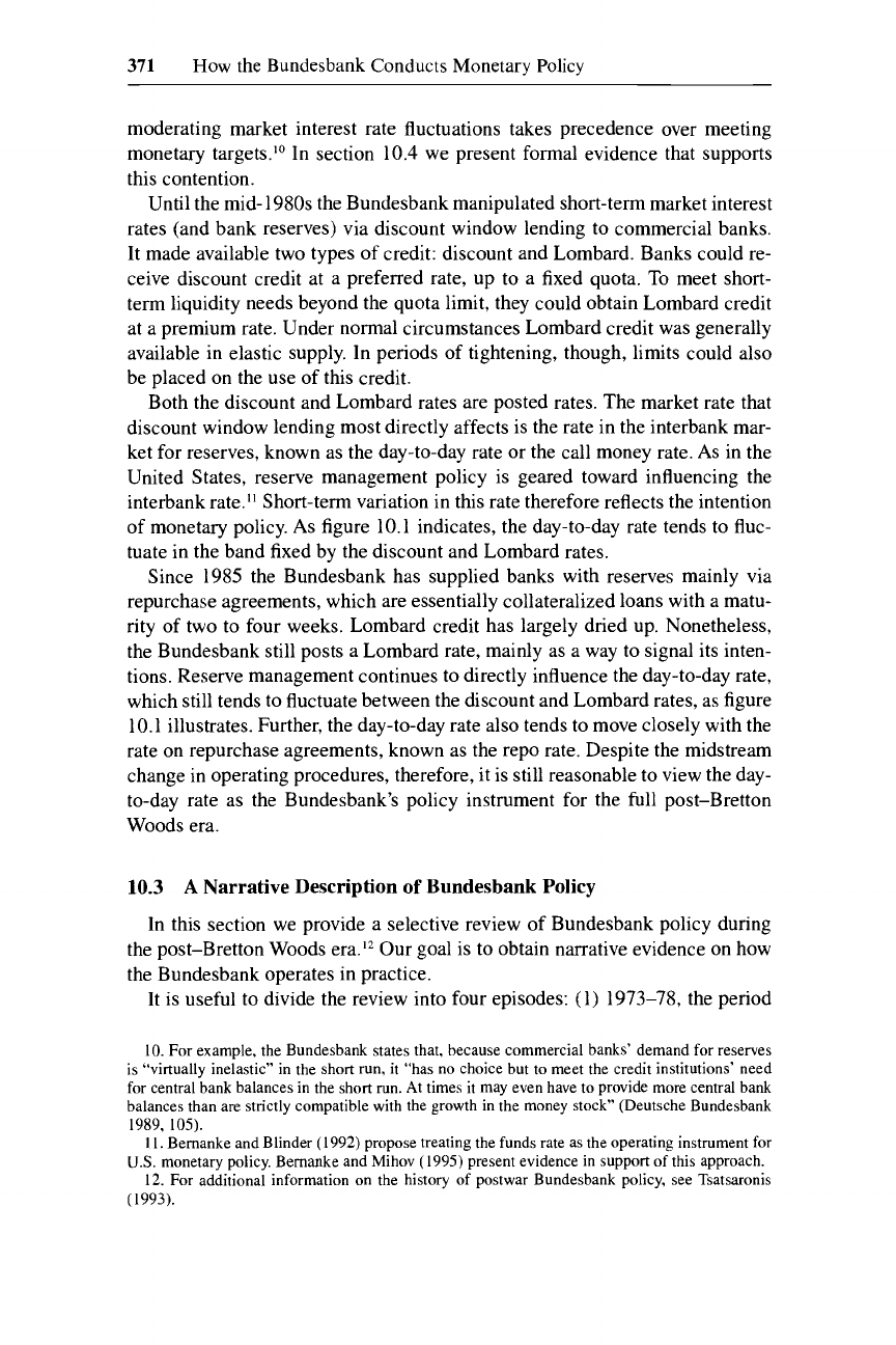
figure 10.1 indicates, the day-to-day rate tends to fluc-
tuate in the band fixed by the discount and Lombard rates.
Since 1985 the Bundesbank has supplied banks with reserves mainly via
repurchase agreements, which
are
essentially collateralized loans with a matu-
rity of two to four weeks. Lombard credit has largely dried up. Nonetheless,
the Bundesbank still posts a Lombard rate, mainly as a way to signal its inten-
tions. Reserve management continues to directly influence the day-to-day rate,
which still tends to fluctuate between the discount and Lombard rates,
as
figure
10.1
illustrates. Further, the day-to-day rate also tends to move closely with the
rate on repurchase agreements, known as the rep0 rate. Despite the midstream
change in operating procedures, therefore, it is still reasonable to view the day-
to-day rate as the Bundesbank’s policy instrument
for
the full post-Bretton
Woods era.
10.3
A
Narrative Description
of
Bundesbank Policy
In this section we provide a selective review of Bundesbank policy during
the post-Bretton Woods era.12 Our goal is to obtain narrative evidence on how
the Bundesbank operates in practice.
It is useful to divide the review into four episodes:
(1)
1973-78, the period
10.
For
example, the Bundesbank states that, because commercial banks’ demand for reserves
is “virtually inelastic” in the short run, it “has no choice but to meet the credit institutions’ need
for
central bank balances in the short
run.
At times
it
may
even
have to provide more central bank
balances than
are strictly compatible with the growth in the money stock” (Deutsche Bundesbank
1989,
105).
I
1. Bernanke and Blinder (1992) propose treating the funds rate
as
the operating instrument
for
U.S.
monetary policy, Bernanke and Mihov (1995) present evidence
in
support of this approach.
12. For
additional information on the history
of
postwar Bundesbank policy,
see
Tsatsaronis
(1993).

372
Richard Clarida and Mark Gertler
16.00
14.00
12.00
1.0.00
8.00
6.00
4.00
2.00
0.00
'
73 76 79
82 85 88 91
94
Fig.
10.1
German short-term interest rates
immediately after Bretton Woods was abandoned and after the first major oil
shock occurred; (2) 1979-83, when the second major oil shock occurred and
the United States tightened monetary policy; (3) 1983-89, the era of stagnation
and late recovery in West Germany; (4) 1990-93, the early years of reunifica-
tion. After a brief discussion
of
each episode, we summarize the key lessons
about the conduct
of
Bundesbank policy.
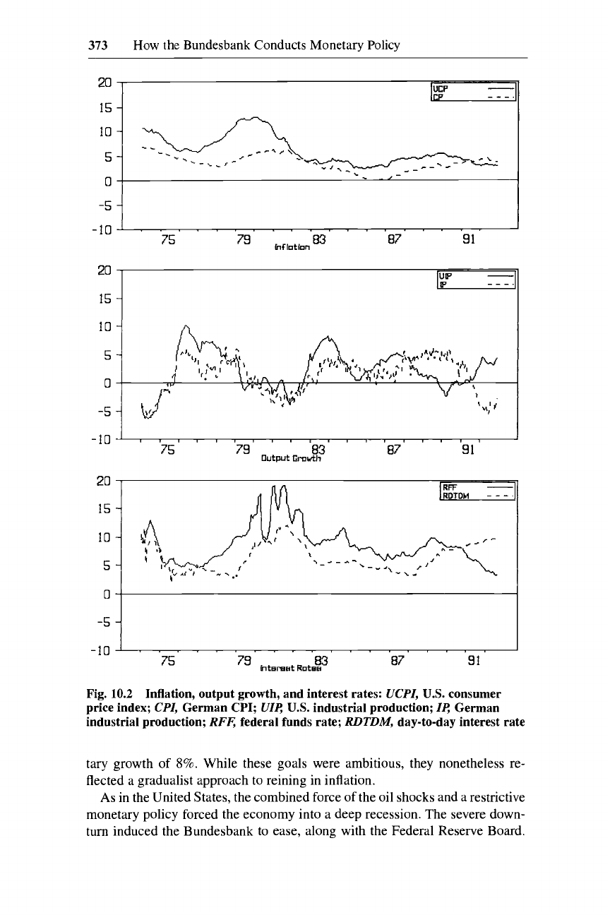
To aid the discussion, we refer (often implicitly) to figure 10.2, which plots
consumer price index
(CPI)
inflation, the growth rate
of
industrial production,
and the day-to-day rate, all for West Germany. To provide a benchmark, the
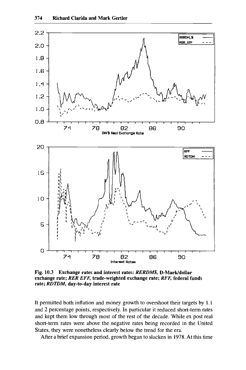
figure also plots the analogous variables for the U.S. economy. In addition
figure 10.3 plots the behavior
of
both the real D-marMdollar exchange rate,
and the trade weighted exchange rate.
10.3.1 1973-1978
Shortly after it was freed from its obligations under Bretton Woods in early
1973, the Bundesbank raised short-term interest rates dramatically in order to
curtail steadily rising inflation. On a number
of
occasions during this period
it
publicly announced a commitment to maintaining
d
tight monetary policy until
inflation was under control (Tsatsaronis 1993). Unfortunately, later in the year
came the first major oil shock. Thus, despite a restrictive policy through most
of 1973, inflation climbed above 7% by the end
of
1974. Though below the
nearly double-digit level reached
in
the United States, this rate was clearly high
by West German standards.
The Bundesbank continued to signal its intent to combat inflation. By the
end of 1974, it had the system
of
inflation and monetary targeting intact. It
announced a target rate of inflation for 1975 of 4.5% and a target rate of mone-
373
How
the Bundesbank Conducts Monetary Policy
15
-
-
UP
P
I
15
-I
RFF
-
RDTDM
-
-
-'
20
-5
1
87
91
-10'
'.
' ' '
*
'
''
'
'
'
'.
. . . .
'
83
79
ht6lmst Rot6H
75
Fig.
10.2
Inflation, output growth, and interest rates: UCPZ,
U.S.
consumer
price index; CPZ, German
CPI;
UZe
U.S.
industrial production;
Ze
German
industrial production;
RFe
federal funds rate;
RDTDM,
day-to-day interest rate
tary growth
of
8%.
While these goals were ambitious, they nonetheless re-
flected a gradualist approach to reining in inflation.
As
in the United States, the combined force of the oil shocks and
a
restrictive
monetary policy forced the economy into a deep recession. The severe down-
turn induced the Bundesbank to ease, along with the Federal Reserve Board.
374
Richard Clarida and Mark Gertler
2.2
2
.o
1.8
1.6
1.4
1.2
1
.o
20
15
10
5
Fig.
10.3
Exchange rates and interest rates:
RERDM$,
D-MarWdollar
exchange rate;
RER EFF,
trade-weighted exchange rate;
RFF,
federal funds
rate;
RDTDM,
day-to-day interest rate
It permitted both inflation and money growth to overshoot their targets by
1.1
and
2
percentage points, respectively. In particular it reduced short-term rates
and kept them low through most of the rest of the decade. While ex post real
short-term rates were above the negative rates being recorded in the United
States, they were nonetheless clearly below the trend for the era.
After a brief expansion period, growth began to slacken in
1978.
At
this time

375
How
the Bundesbank Conducts Monetary Policy
the Bundesbank cited an appreciating mark to justify continued easing. In ef-
fect the Bundesbank was easing rates to stimulate a softening real economy.
While it is not always so forthcoming, it has acknowledged that concern for
the real economy influenced its behavior during this period.13
10.3.2 1979-1 983
Just prior to 1979, macroeconomic conditions in West Germany were more
favorable than in the United States. Output growth was roughly similar. While
the inflation rate was still stubbornly high by West German standards, it was
well below the U.S. inflation rate. Fortunes were reversed, however, in the eight
years after.
The first oil shock and the subsequent shift in U.S. monetary policy ushered
in a return to tight money. The Bundesbank was committed to avoiding (what
it viewed as) its earlier mistake of largely accommodating the increases in oil
prices during 1973 and 1974 (Tsatsaronis 1993). In addition the sharp rise in
U.S. interest rates precipitated a sharp and steady depreciation of the mark
relative to the dollar that lasted until 1985.
The Bundesbank responded to these events by raising the day-to-day rate
from about 3% in 1979 to about 12% in the first quarter of 1981. In terms of
basis points, this increase was similar in magnitude to the rise in the U.S. funds
over same period. Ex post real rates rose sharply, as they did in the United
States.
Again, its pragmatic side showed through: the Bundesbank raised the target
rate of inflation from 3% in 1979 to 4% in 1980. And it still permitted inflation
to overshoot its target by 1.3%. The weakening of the real economy at the time
was again apparently a factor in the Bundesbank’s decision making. For the
next two years it continued the gradualist policy, tolerating above-target infla-
tion in order to avoid further weakening a recessionary economy.
From the period of peak inflation to the beginning of 1983, the contraction
in real activity in West Germany was of similar magnitude to that in the United
States. On the other hand, the drop in inflation over the same time interval was
far more dramatic in the United States. At the start of the period the U.S. infla-
tion rate was nearly double that in West Germany. By the end it was roughly
equal. These facts correspond closely to Ball’s observation (1994) that the sac-
rifice ratio in Germany actually exceeds its counterpart for the United States.
Many have found this outcome surprising. Underlying this view is the belief
that the Bundesbank’s reputation for fighting inflation should have made the
transition to lower inflation less painful in this country relative to other coun-
tries at the time. This in turn raises the possibility that the practical gains from
establishing credibility in fighting inflation may not be substantial. Fully re-
13.
The Bundesbank states that when the D-mark appreciated “excessively” in
1978
(and also
in 1986-87),
it
felt “forced to pursue a more expansionary monetary policy and allow interest rate
reductions
. .
.
which led to an overshooting
of
the monetary target. Otherwise the appreciation
shock would have too much for the economy, while inflationary pressures were being moderated
by the appreciation” (Deutsche Bundesbank 1989,
103).

376
Richard Clarida and
Mark
Gertler
solving this issue is well beyond the scope of this paper, though we return
to
the matter later.
For now we simply note two considerations. First, the sacrifice ratio could
be highly nonlinear in practice, something for which the Ball calculation does
not allow. One could imagine why trying to move an economy from
6%
to 2%
inflation might result in greater short-run output loss than, say, trying to move
it from 10% to
6%.
This nonlinear relationship could resolve at least some of
the differences in the
U.S.
and West German experience.
Second, and somewhat related, at the beginning of 1979 the public percep-
tion of the Bundesbank’s commitment to reduce inflation below
56%
may
have been more ambiguous than it is today.
As
we have discussed, the Bundes-
bank pursued
a
relatively lax monetary policy in the roughly four years prior
to the shift to tightening. Again, we turn to this issue later.
10.3.3 1983-1989
While the U.S. economy staged a strong recovery following the 1981-82
recession, the same was not true of the West German economy. Growth was
slightly below trend in 1983 and only slightly above trend in 1984 and 1985.
The unemployment rate continued to rise steadily, reaching 9.3% in 1985. On
the other hand, a product of the weak economy was receding inflation. Inflation
was below target from 1983 to 1985. During this period the Bundesbank re-
turned short-term nominal rates to slightly above pre-1979 levels. Lower infla-
tion, however, implied significantly higher real interest rates than during the
late 1970s.
As
we show in section 10.5, real rates during this period hovered
slightly around and above long-run equilibrium.
Why the West German economy (along with the rest of the European econ-
omy) performed poorly over this period is
a
complex issue, another that is well
beyond the paper’s scope. It is plausible that high real interest rates were a
factor. Real rates were similarly high in the United States at this time. The
United States, however, had shifted to an expansionary fiscal policy. The same
kind
of
fiscal stimulus was not present in West Germany.
Another often-cited possibility is that the German economy was experienc-
ing structural labor market problems at this time (e.g., Kahn and Jacobson
1989). This would imply that the stagnant economy was due mainly to supply-
side problems, that
is,
declines in capacity output. It is true that real wages
grew rapidly from 1973 through 1989. The period 1982-85, though, does not
appear to have been a period of rapid wage growth. While we do not claim
to
resolve the issue, later we examine more carefully the behavior of output rela-
tive to capacity and real interest rates over this period.
In
mid-1984 the United States began a systematic reduction of the funds rate
in an effort, among other things, to reduce the value of the dollar. In early 1985
the mark began a steady appreciation against the dollar that lasted through early
1988. In response to the appreciating mark, the real economy weakened. Out-
put growth declined over 1986 and 1987. Inflation fell below the
2%
target.
The weak economy prompted the Bundesbank to once again demonstrate
377
How
the Bundesbank Conducts Monetary Policy
its flexibility in both actions and language. Citing an appreciating mark, the
Bundesbank eased short-term interest rates. Real short-term rates fell, though
not to the levels of the mid- to late 1970s. Following the easing, output growth
picked up
in
1989. A strong recovery finally materialized.
10.3.4 1990-1993
The robust output growth in West Germany that began in 1989 continued
through reunification in 1990, and into 1991. The unemployment rate fell over
this period, for the first time in a decade.
Reunification of course introduced new complexities for monetary manage-
ment. At the time, though, the Bundesbank had two particular concerns. First,
the robust expansion led inflation to accelerate above target in 1991. Second,
the one-for-one currency exchange with East Germany led to a whopping 13%
increase in the M3 aggregate within a single month. The jump complicated the
problem of monetary targeting. Of greater concern to the Bundesbank was the
possible consequence for inflation, especially given the large implicit subsidy
in the currency swap.
Fear of renewed inflation induced the Bundesbank to aggressively tighten.
It raised short-term nominal rates above 9%. Real rates rose to the high levels
of the early 1980s. For the first time since Bretton Woods, both nominal and
real rates in Germany were higher than in the United States. One casualty of
the tightening was the EMS. The
EMS
collapsed in September 1992 due in
large part to the unwillingness of other members, especially the United King-
dom, to keep their interest rates in line with the soaring German rates. The
tightening also had predictable effects on the Germany economy. Due at least
in
part to monetary policy, output plummeted. West German industrial produc-
tion dropped 15% from January 1992 through September 1993. And the unem-
ployment rate rose nearly 3 percentage points over this same period.
The recessionary economy prompted the Bundesbank to ease rates. The eas-
ing, however, was modest. While both nominal and real rates declined, the
level of the real rate remained high relative to earlier periods
of
downturns. We
return to this issue in section 10.5.
10.3.5
Bundesbank Policy in Practice: Summary of the Narrative Evidence
The Bundesbank aggressively raises short-term interest rates in response to
perceived inflationary pressures. An exception was the period 1975-78, when
it maintained subnormal short-term real interest rates while inflation was above
the desired trend, much as the United States was doing at the same time. There
is some suggestion, even
in
official Bundesbank publications, that the experi-
ence with stagflation during this period explains why the Bundesbank has been
more vigilant about controlling inflation in the years since then. The German
experience suggests that, once inflation starts to persist above trend, it is diffi-
cult to bring down costlessly, even for a central bank with the reputation of the
Bundesbank. Again, there is a clear parallel with the U.S. experience.
In its actions, if not its public pronouncements, the Bundesbank also clearly
378
Richard Clarida and Mark
Gertler
takes into account the performance of the real economy. While it desires to
control inflation, it will not do
so
at
any cost. Conversely, a soft economy with
an appreciating D-mark normally induces the Bundesbank to ease.
A
case can
be made, though, that in recent years the easings have been more modest rela-
tive to the overall condition of the economy.
What role does targeting play in the day-to-day formulation of policy? The
targets do not define a rigid rule for money growth. In the period
1975-93
the
Bundesbank failed to meet its money-growth target in
9
of
19
possible in-
stances. Rather, as the Bundesbank has made clear on numerous occasions, the
targets are to be viewed as guidelines. They provide the policy decision with a
clear reference point. The Bundesbank is free to deviate from this reference
point. But it is expected to explain the circumstances that lead it to do
so.
In
this way the targets place discipline on the policymaking process.
The pattern of deviations from the inflation and money-growth targets are
in our view symptomatic of the implicit stabilization component in the Bunde-
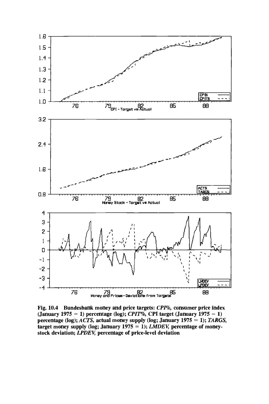
sbank policy rule. The top panel of figure
10.4
plots the target price level (in
logarithms) implied by the sequence of target inflation rates, relative to the
actual price level. The middle panel does the same for the money supply. Note
that during the high inflation of the late
1970s
and early
1980s
the Bundesbank
persistently accommodated overshooting of the price target by simply rebench-
marking the path for the target price each year. That is, it made no attempt to
target a long-term path for the price level, presumably because it feared the
consequences for the real economy.
The bottom panel plots the percentage deviation of each variable from its
target. Note that between
1979
and
1989
the two series are almost mirror im-
ages of one another. This strong negative relationship between the price-level
and money-stock deviations also reveals an element of stabilization within the
policy rule. Generally speaking, when the price level significantly overshoots
its target, the Bundesbank pursues a contractionary policy that tends to push
the money supply below target.
As
we have been emphasizing, the Bundes-
bank’s toleration of this overshooting is evidence of a stabilization concern. In
a way, the simultaneous undershooting of the money-growth target provides it
with a formal justification not to tighten further.
Conversely, in periods where the price level is significantly under target, the
Bundesbank often pushes money growth above target. The undershooting of
the price target presumably gives it leeway to ease monetary policy. In these
situations, as we have discussed, it usually cites an overvalued D-mark to ratio-
nalize its aims.
10.4
Identifying the Bundesbank’s Policy Reaction Function:
A
Structural VAR Approach
In section
10.3
we developed a set of informal conclusions about the nature
of Bundesbank policy. In this section and the next we probe the issues further
1.6
1.5
1.4
1,3
1.2
1.1
1
.o
3'2
I
2.4
1.6
0.8
Fig. 10.4 Bundesbank money and price targets:
CPZ%,
consumer price index
(January 1975
=
1) percentage (log);
CPZT%,
CPI target (January 1975
=
1)
percentage
(log);
ACTS,
actual money supply (log; January 1975
=
1);
TARGS,
target money supply (log; January 1975
=
1);
LMDEY
percentage
of
money-
stock deviation;
LPDEY
percentage
of
price-level deviation
380
Richard Clarida and Mark
Gertler
by estimating policy reaction functions. Based on the previous discussion, we
take as the Bundesbank's policy instrument the day-to-day interest rate. Our
goal then is to identify an empirical relationship that is useful for characteriz-
ing how the Bundesbank adjusts the short-term rate over time.
In general, identifying
a
reaction function for central bank policy involves
confronting two basic complex issues. First, one has to take
a
stand on the set
of information to which the central bank responds. The central bank may have
a primary goal of stabilizing inflation and output, for example. But it may (and
in general does) take account of
a
far broader set of information than simply
inflation and output. Additional information may be useful for forecasting fu-
ture inflation and future output. Good examples are exchange rates and com-
modity prices. Also, the central bank may make use of intermediate targets
such
as
the exchange rate or the money supply, either because it cannot directly
observe current inflation and current output or because it desires some kind
of
commitment device. Indeed, the discussion in section
10.3
suggests that both
the money supply and exchange rates are factored into Bundesbank policy de-
cisions in an important way.
Second, there is a problem of simultaneity between the policy instrument
and the information set. The Bundesbank may adjust short-term interest rates
in light of news about exchanges rates, for example. But, certainly, the change
in the short-term rate will feed back into the behavior of the exchange rate.
We take
a
two-pronged approach to the identification problem. The first
prong, which we pursue in this section, is to estimate
a
policy reaction function
for the day-to-day rate that is derived from
a
structural VAR model of the Ger-
man macroe~onomy.'~ With this reaction function we can characterize in
a
fairly general way how the Bundesbank adjusts policy in response to distur-
bances, such
as
supply shocks, changes in
US.
monetary policy, exogenous
exchange rate shifts, and
so
on. The benefit of this approach is that we can
address the identification issues by employing relatively few
a
priori restric-
tions (at least relative to other approaches). The cost is that because the esti-
mated reaction function includes all the variables in the VAR it is difficult to
interpret. Therefore, in section
10.5
we move on to the second prong, which
involves imposing additional structure on the basic empirical model developed
in this section.
10.4.1
The General Ident$cation
Strategy
Let
y,
be
a
vector of macroeconomic variables and
e,
be an associated vector
of structural disturbances. The elements of
e,
are mutually orthogonal iid dis-
turbances. They are structural shocks in the sense that they are the primitive
Using
a
Structural VAR to Identify Policy Rules
14.
For
some useful descriptions
of
the structural
VAR
methodology, see Blanchard 1989;
Cali
1992; Sims and Zha 1994; Kim and Roubini 1995; Bernanke and Mihov 1995.
381
How
the
Bundesbank Conducts Monetary Policy
exogenous disturbances to the economy.
A
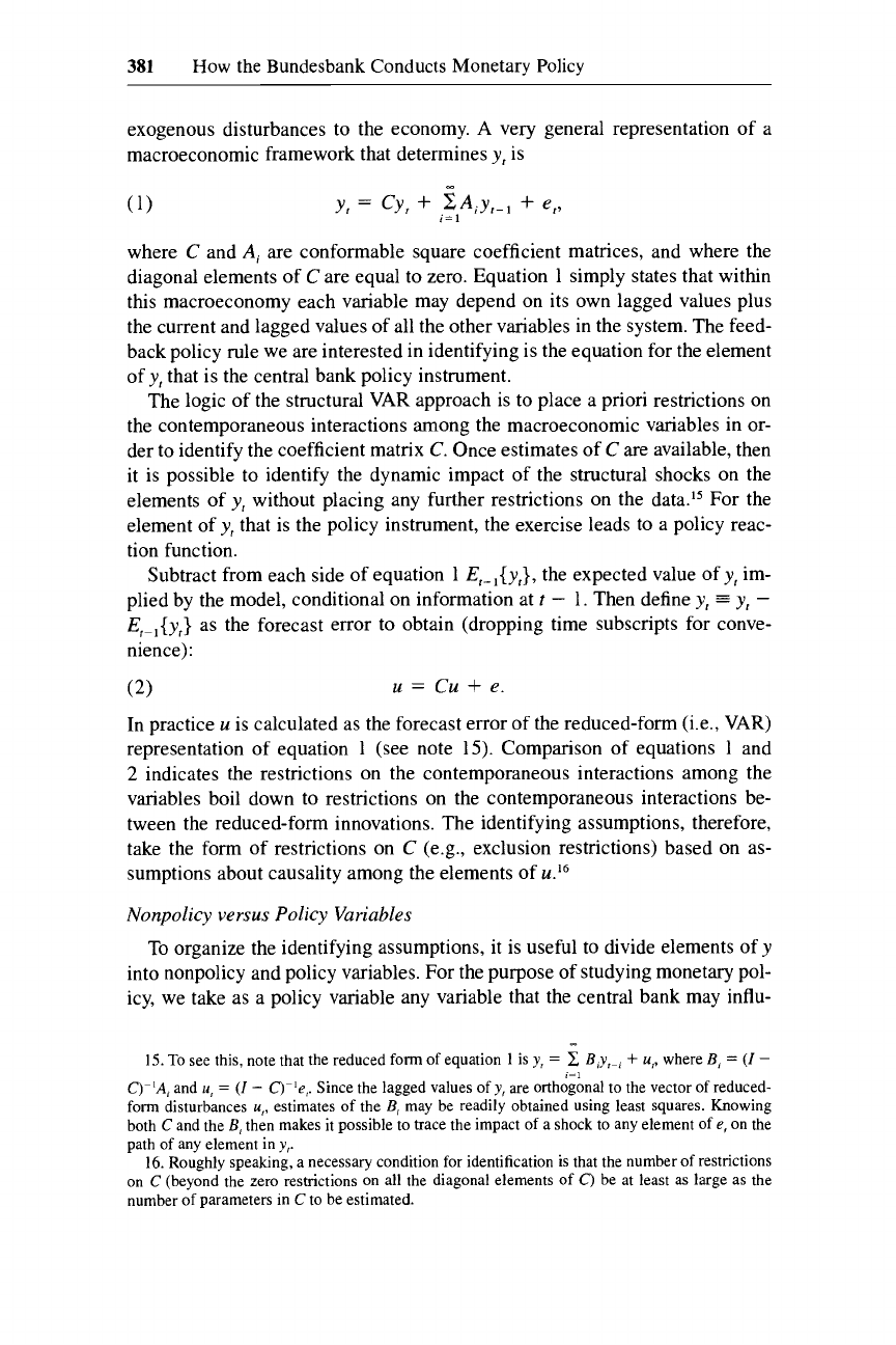
very general representation of a
macroeconomic framework that determines
y,
is
y,
=
Cy,
+
~A;Y,-~
+
e,,
(1)
where
C
and
Ai
are conformable square coefficient matrices, and where the
diagonal elements
of
C
are equal to zero. Equation
1
simply states that within
this macroeconomy each variable may depend on its own lagged values plus
the current and lagged values of all the other variables in the system. The feed-
back policy rule we are interested in identifying is the equation for the element
of
y,
that is the central bank policy instrument.
The logic of the structural VAR approach
is
to place a priori restrictions on
the contemporaneous interactions among the macroeconomic variables in or-
der
to
identify the coefficient matrix
C.
Once estimates of
C
are available, then
it is possible to identify the dynamic impact of the structural shocks on the
elements of
y,
without placing any further restrictions on the data." For the
element of
y,
that is the policy instrument, the exercise leads to a policy reac-
tion function.
Subtract from each side of equation
1
E,-l{y,},
the expected value of
y,
im-
plied by the model, conditional on information at
t
-
1.
Then define
y,
=
y,
-
E,-,(y,}
as
the forecast error to obtain (dropping time subscripts for conve-
nience):
u
=
Cu
+
e.
(2)
In practice u is calculated as the forecast error of the reduced-form (ie., VAR)
representation of equation
1
(see note 15). Comparison
of
equations
1
and
2
indicates the restrictions on the contemporaneous interactions among the
variables boil down
to
restrictions on the contemporaneous interactions be-
tween the reduced-form innovations. The identifying assumptions, therefore,
take the form of restrictions on
C
(e.g., exclusion restrictions) based on as-
sumptions about causality among the elements of
u.16
Nonpolicy
versus
Policy
Variables
To
organize the identifying assumptions, it is useful to divide elements of
y
into nonpolicy and policy variables.
For
the purpose of studying monetary pol-
icy, we take as a policy variable any variable that the central bank may influ-
-
i=
I
15.
To
see
this, note that the reduced form of equation
1
is
y,
=
x
BJ-,
+
u,,
where
B,
=
(I
-
C)-'A,
and
u,
=
(I
-
C)-'e,.
Since the lagged values of
y,
are orthogonal
to
the vector of reduced-
form disturbances
u,,
estimates of
the
B,
may be readily obtained using least squares. Knowing
both
C
and the
B,
then makes it possible to trace the impact of a shock to any element of
e,
on the
path of any element in
y,.
16.
Roughly speaking, a necessary condition for identification is that the number of restrictions
on
C
(beyond the
zero
restrictions on all the diagonal elements of
C)
be at least as large as the
number of parameters in
C
to be estimated.
E=1
382
Richard Clarida and
Mark
Gertler
ence within the current period (e.g., within the current month). This definition
thus includes not only the central bank's direct policy instrument (e.g., the day-
to-day interest rate), but also observable "jump" variables such
as
the exchange
rate, over which it exerts indirect influence within the period. Due to the
within-period simultaneity, the central bank is effectively choosing values
of
all the variables that move contemporaneously. Presumably, when the central
bank adjusts the short-term interest rate, for example, it takes into account the
implied contemporaneous reaction of the exchange rate.
The dual implication
of
our classification scheme is that nonpolicy variables
respond only with
a
lag to movements in the policy variables. Output may react
over time to a shift in interest rates, for example, but due to adjustment costs
and
so
on, it does not respond instantaneously. From the standpoint of identi-
fication, innovations in the nonpolicy variables are exogenous to the innova-
tions in the policy
variable^.'^
To identify the equation for the policy instru-
ment, therefore, we need to worry only about addressing the possible
contemporaneous simultaneity among the policy variables (e.g., how the day-
to-day rate responds to the exchange rate and vice versa).
10.4.2
The Empirical Model
Variables
We use eight variables to describe the German macroeconomy. Five are non-
policy variables. Of these, three are meant to characterize the state of the Ger-
man economy: industrial production
(ip),
retail sales
(ret),
and the consumer
price level
(p).
The two others reflect important external factors that influence
the German economy: real commodity prices
(cp)
(meant to capture supply
shocks) and the
U.S.
federal funds rate
(8).
The three Bundesbank policy variables are the day-to-day (i.e., short-term)
interest rate
(rs);
the real money supply
(m)
(specifically the broad money ag-
gregate M3 divided by the price level), and the real D-mark/dollar exchange
rate
(er).
We treat the short-term interest rate
as
the Bundesbank's policy in-
strument, for reasons discussed in section 10.2.3.
17. In particular the contemporaneous exogeneity of the nonpolicy variables implies a set of
useful exclusion restrictions on the coefficient matrix
C
in equation
2.
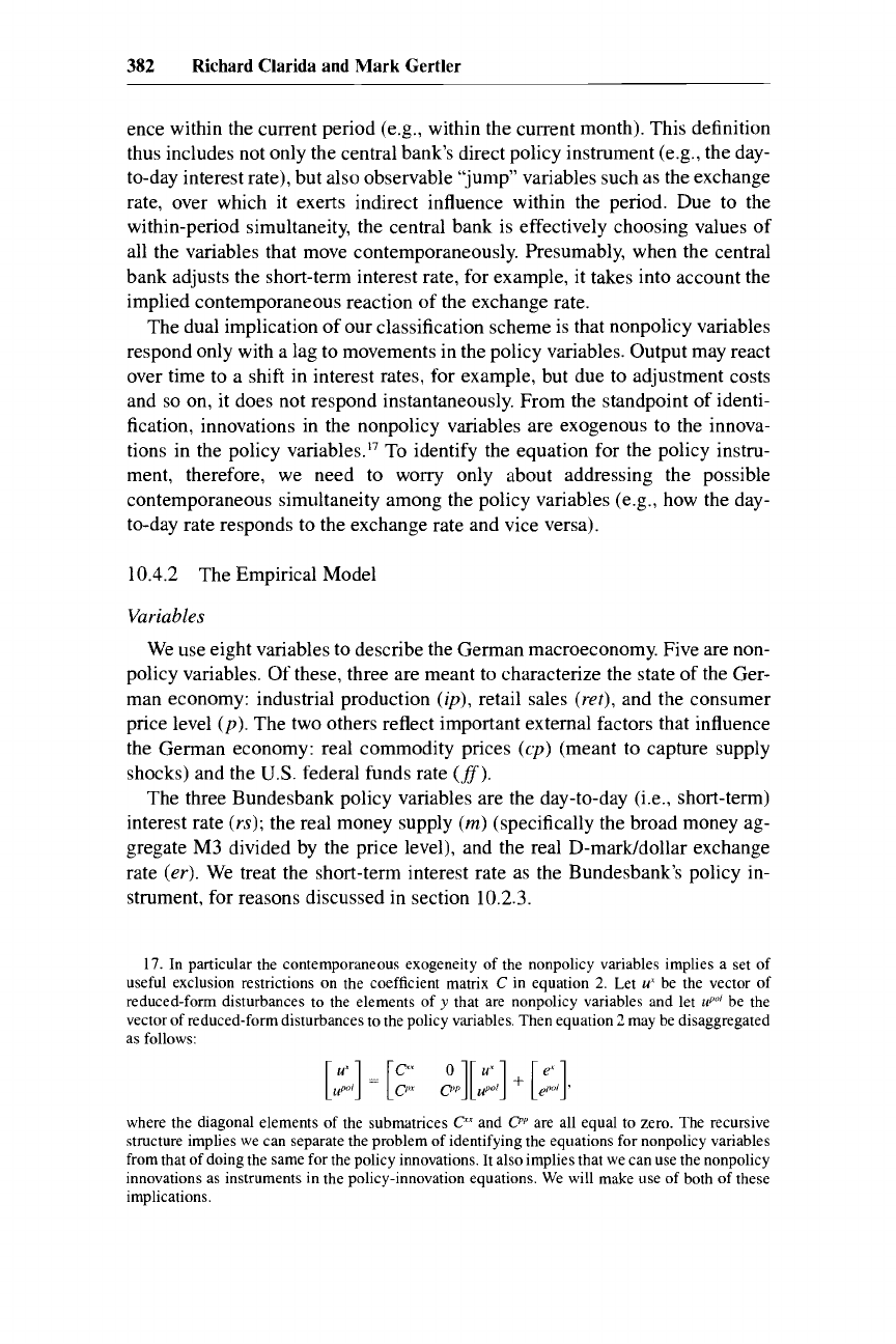
Let u* be the vector of
reduced-form disturbances to the elements of
y
that are nonpolicy variables and let
up<''
be the
vector of reduced-form disturbances to the policy variables. Then equation
2
may be disaggregated
as follows:
where the diagonal elements
of
the submatrices
P
and
CP''
are all equal
to
zero.
The recursive
structure implies we can separate the problem of identifying the equations for nonpolicy variables
from that of doing the same for the policy innovations.
It
also implies that we can use the nonpolicy
innovations as instruments in the policy-innovation equations. We will make
use
of
both
of
these
implications.
383
How
the Bundesbank Conducts Monetary Policy
The real money supply and real exchange rate fit our policy-variable classi-
fication, since the Bundesbank can quickly influence these variables (via its
choice of the short-term interest rate), and because its choice of interest rates
presumably is influenced by these variables.'8 We use the D-marWdollar rate
since our reading of the narrative evidence suggests that it is this exchange rate
that has had the the most influence over Bundesbank policy.
Identifying
Assumptions
the reduced-form innovations are as follows:
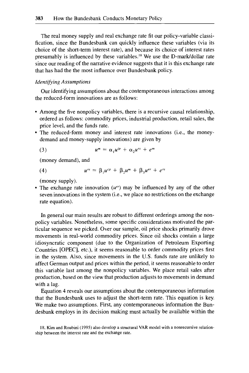
Our identifying assumptions about the contemporaneous interactions among
Among the five nonpolicy variables, there is a recursive causal relationship,
ordered as follows: commodity prices, industrial production, retail sales, the
price level, and the funds rate.
The reduced-form money and interest rate innovations (i.e.,
the
money-
demand and money-supply innovations) are given by
(3)
(money demand), and
(4)
(money supply).
The exchange rate innovation
(u")
may be influenced by any of the other
seven innovations in the system (i.e., we place
no
restrictions on the exchange
rate equation).
urn
=
a,uiP
+
a2urS
+
em
u"
=
p,ucp
+
P2um
+
P3uer
+
ers
In general our main results
are
robust to different orderings among the non-
policy variables. Nonetheless, some specific considerations motivated the par-
ticular sequence we picked. Over our sample, oil price shocks primarily drove
movements in real-world commodity prices. Since oil shocks contain a large
idiosyncratic component (due to the Organization of Petroleum Exporting
Countries [OPEC], etc.), it seems reasonable to order commodity prices first
in the system. Also, since movements in the
U.S.
funds rate are unlikely to
affect German output and prices within the period, it seems reasonable to order
this variable last among the nonpolicy variables. We place retail sales after
production, based on the view that production adjusts to movements in demand
with a lag.
Equation
4
reveals our assumptions about the contemporaneous information
that the Bundesbank uses to adjust the short-term rate. This equation is key.
We make two assumptions. First, any contemporaneous information the Bun-
desbank employs in its decision making must actually be available within the
18.
Kim and Roubini
(1995)
also develop a structural VAR model with a nomecursive relation-
ship between the interest rate and the exchange rate.
384
Richard Clarida and
Mark
Gertler
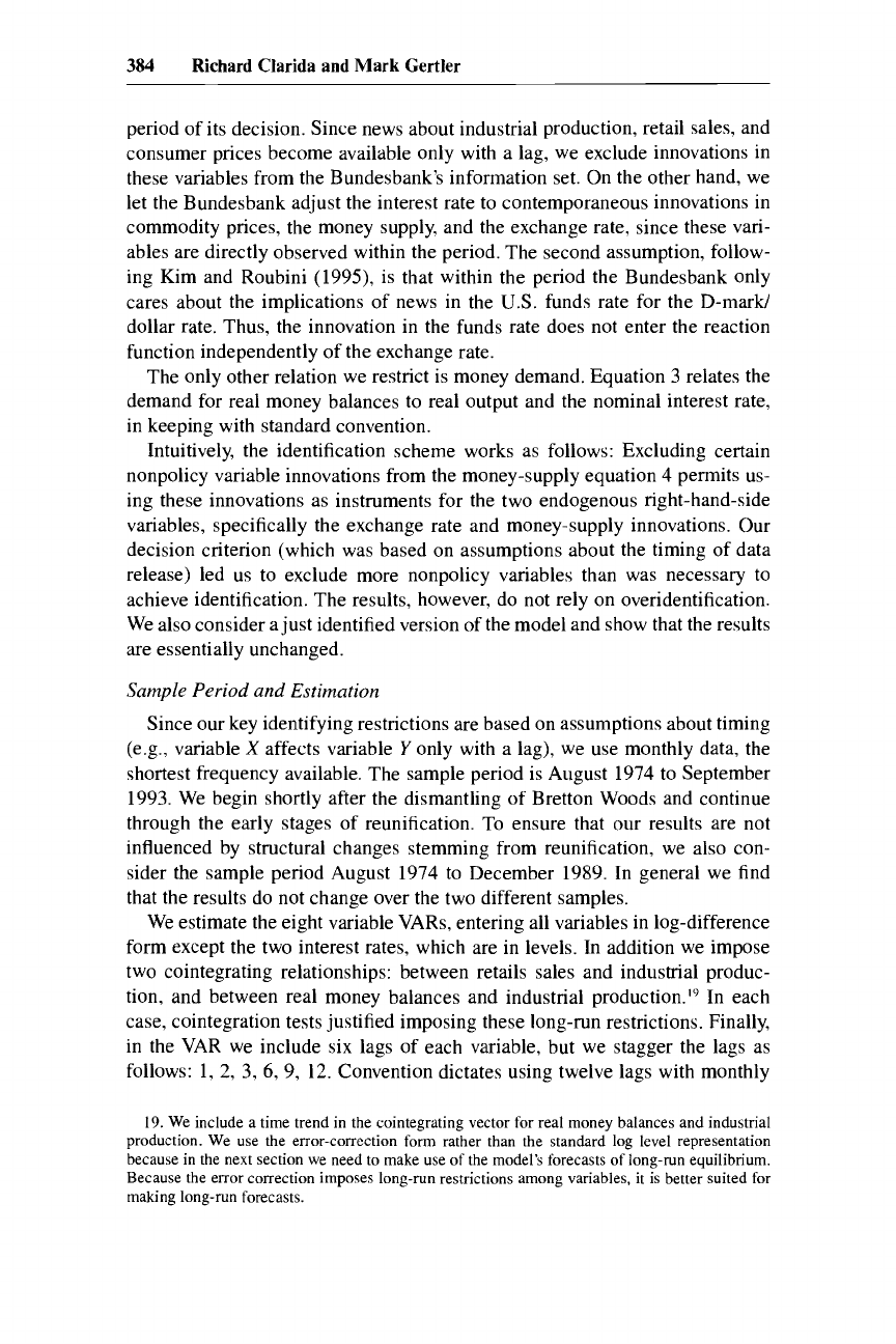
period of its decision. Since news about industrial production, retail sales, and
consumer prices become available only with
a
lag, we exclude innovations in
these variables from the Bundesbank's information set. On the other hand, we
let the Bundesbank adjust the interest rate to contemporaneous innovations in
commodity prices, the money supply, and the exchange rate, since these vari-
ables are directly observed within the period. The second assumption, follow-
ing Kim and Roubini (1995), is that within the period the Bundesbank only
cares about the implications of news in the
U.S.
funds rate for the D-mark/
dollar rate. Thus, the innovation in the funds rate does not enter the reaction
function independently
of
the exchange rate.
The only other relation we restrict is money demand. Equation 3 relates the
demand for real money balances to real output and the nominal interest rate,
in keeping with standard convention.
Intuitively, the identification scheme works as follows: Excluding certain
nonpolicy variable innovations from the money-supply equation
4
permits us-
ing these innovations
as
instruments for the two endogenous right-hand-side
variables, specifically the exchange rate and money-supply innovations. Our
decision criterion (which was based on assumptions about the timing of data
release) led us to exclude more nonpolicy variables than was necessary to
achieve identification. The results, however, do not rely on overidentification.
We also consider
a
just identified version of the model and show that the results
are essentially unchanged.
Sample Period and Estimation
Since our key identifying restrictions are based on assumptions about timing
(e.g., variable
X
affects variable
Y
only with
a
lag), we use monthly data, the
shortest frequency available. The sample period is August 1974 to September
1993. We begin shortly after the dismantling of Bretton Woods and continue
through the early stages of reunification. To ensure that our results are not
influenced by structural changes stemming from reunification, we also con-
sider the sample period August 1974 to December 1989. In general we find
that the results
do
not change over the two different samples.
We estimate the eight variable VARs, entering all variables in log-difference
form except the two interest rates, which are in levels. In addition we impose
two cointegrating relationships: between retails sales and industrial produc-
tion, and between real money balances and industrial production.'" In each
case, cointegration tests justified imposing these long-run restrictions. Finally,
in the VAR we include six lags of each variable, but we stagger the lags
as
follows: 1,
2,
3,
6,
9,
12.
Convention dictates using twelve lags with monthly
19.
We include
a
time trend in the cointegrating vector for real money balances and industrial
production. We use the error-corrcction form rather than the standard log level representation
because in the next section we need to make use of the model's forecasts
of
long-run equilibrium.
Because the error correction imposes long-run restrictions among variables, it is better suited for
making long-run forecasts.

385
How
the Bundesbank Conducts Monetary Policy
data to avoid problems of seasonality. However, because the sample period is
short relative to the number of variables and because we also want to use the
model to make long-horizon forecasts in the next section, we opted for a more
parsimonious parameterization.
10.4.3 Results
We are interested in assessing how the Bundesbank adjusts the short-term
interest rate to disturbances to the economy, particularly in light of the narra-
tive evidence developed in section 10.3. We first report evidence on how the
Bundesbank adjusts the day-to-day rates to within-period news. We then ana-
lyze the response of the interest rate over time to various shocks to the econ-
omy. In this way we are able to characterize policy reaction function for the
Bundesbank.
Policy Response
to
Contemporaneous News
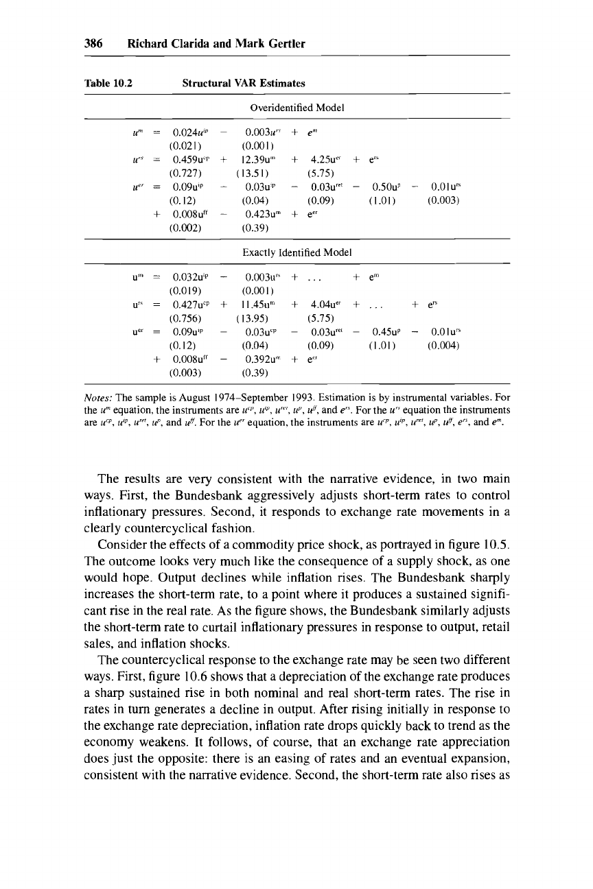
Table 10.2 reports estimates of money-supply equation
4,
which relates the
innovation
in
the interest rate to the innovations in commodity prices, the
money supply, and the exchange rate. The point estimates are as one would
expect. The Bundesbank lets the short-term rate rise in response to news of
increases in inflationary pressures, manifested in either a rise in commodity
prices, a rise in the money supply, or a depreciation of the exchange rate. None
of the news variables is statistically significant, however. This suggests that the
Bundesbank does not try to tightly meet monetary or exchange rate targets
within the month. It also suggests that it is mainly lagged rather than current
information that is fed into the Bundesbank’s policy rule. Within a given month
the Bundesbank tends to maintain a desired short-term rate, given the informa-
tion available at the start of the period.
As
a check that our identification scheme is reasonable, we
also
report the
estimates
of
the two other equations that enter the policy block, the money-
demand and exchange rate relations. In both cases the outcomes are quite sen-
sible. Money demand has a significant negative interest elasticity. An innova-
tion in the funds rate causes the exchange rate to depreciate significantly, while
an innovation in the German short-term rate does the reverse. Finally, a just-
identified version
of
the model yields very similar coefficient estimates for all
three equations.
Dynamic Policy Response
to
Various
Shocks
We next assess how the Bundesbank adjusts the short-term rate over time to
disturbances to the economy,
To
do
so,
we report the response to each of the
eight structural shocks of a subset of four core variables that characterize the
overall state of the economy and policy: industrial production, inflation,
the short-term interest rate, and the real exchange rate. In addition we report
the response
of
the variable that is shocked. Figures
10.5
and 10.6 show the
results, the mean responses of the variables and their
95%
confidence intervals.
386
Richard Clarida and Mark
Gertler
Table
10.2
Structural
VAR
Estimates
Overidentified Model
u"'
=
O.O24u'8
~
0.003~"
+
e"'
(0.021)
(0.001)
u"
=
0.459uLp
+
12.39~"'
+
4.25~"
+
e"
(0.727)
(13.51)
(5.75)
U"
=
0.09u'P
-
0.03u'P
-
0.03~"'
-
0.50uP
-
0.01~"
(0.12) (0.04) (0.09)
(1.01)
(0.003)
(0.002)
(0.39)
+
0.008~~~
-
0.423~"
+
err
Exactly Identified
Model
"1"
=
0.032U'P
(0.019)
u"
=
0.427u'p
(0.756)
uer
=
0.09u'p
(0.12)
+
0.008u"
(0.003)
-
0.003~"
+
,
. .
+
em
+
11.45~"
+
4.04~"
+
.
.
.
+
erb
(0.001)
(13.95) (5.75)
-
0.03u'P
-
0.03~"'
-
0.45uP
-
0.01~"
(0.04)
(0.09)
(1.01)
(0.004)
(0.39)
-
0.392~'"
+
e"
Notes:
The sample is August 1974-September 1993. Estimation is by instrumental variables.
For
the
urn
equation, the instruments are
uC~',
u'p,
u"",
up,
&',
and
e".
For
the
u"
equation the instruments
are
ucp,
u'~,
ur',
up,
and
&'.
For
the
up"
equation, the instruments are
ucp,
u'p,
ZP',
up,
Un,
e",
and
em.
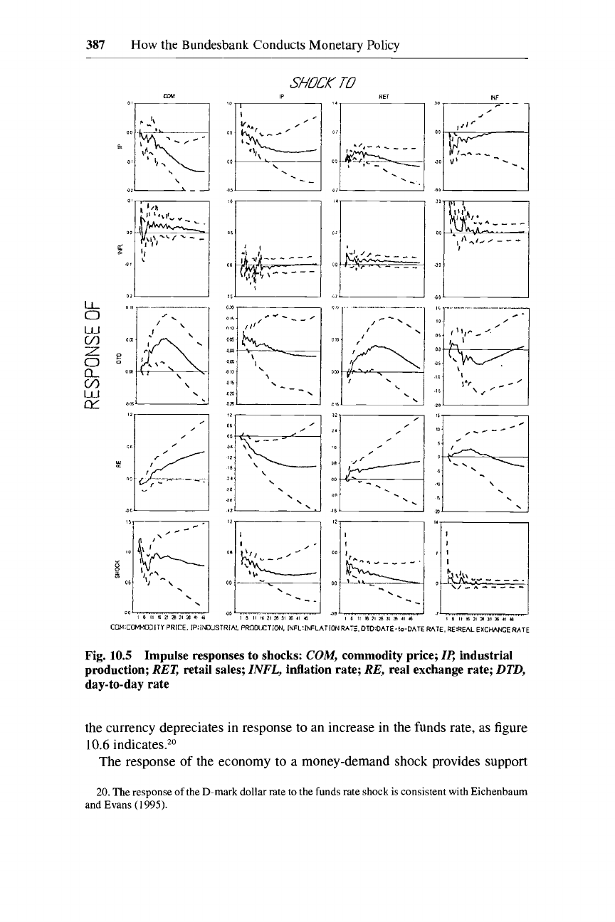
The results are very consistent with the narrative evidence, in two main
ways. First, the Bundesbank aggressively adjusts short-term rates to control
inflationary pressures. Second, it responds to exchange rate movements in a
clearly countercyclical fashion.
Consider the effects
of
a commodity price shock, as portrayed in figure
10.5.
The outcome looks very much like the consequence of a supply shock,
as
one
would hope. Output declines while inflation rises. The Bundesbank sharply
increases the short-term rate, to a point where it produces a sustained signifi-
cant rise in the real rate. As the figure shows, the Bundesbank similarly adjusts
the short-term rate to curtail inflationary pressures in response to output, retail
sales, and inflation shocks.
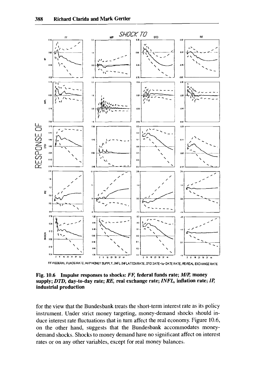
The countercyclical response to the exchange rate may be seen two different
ways. First, figure
10.6
shows that a depreciation of the exchange rate produces
a sharp sustained rise in both nominal and real short-term rates. The rise in
rates in turn generates a decline in output. After rising initially in response to
the exchange rate depreciation, inflation rate drops quickly back to trend
as
the
economy weakens. It follows, of course, that an exchange rate appreciation
does just the opposite: there is an easing
of
rates and an eventual expansion,
consistent with the narrative evidence. Second, the short-term rate also rises as
387
How
the Bundesbank Conducts Monetary Policy
IP
RFl
SHDCK
727
IT-?--
1
-I-
C0M:CD~ITY PRICE. IP:IWUSlRlhL PRNAJCTION. 1NFL:INFLATION
RAX
DT0:OATE-C-DATE RATE, RE:REAL
EXCHANGE
RATE
Fig.
10.5
Impulse responses to shocks:
COM,
commodity price;
Il:
industrial
production;
RET,
retail sales;
INFL,
inflation rate;
RE,
real exchange rate;
DTD,
day-to-day rate
the currency depreciates in response
to
an increase in the funds rate, as figure
10.6
indicates.*"
The response of the economy to a money-demand shock provides support
20.
The
response
of
the D-mark dollar rate
to
the funds rate shock is consistent with Eichenbaum
and Evans
(1
995).
388
Richard Clarida and Mark Gertler
03,
I
FF:FEOERAL FUNDS
RATE.
MIP:MCNEY
SUPPiY.
1ML:INLATICNRATE. DiJ:MTE-Io-OATE
RATE,
REREAL
EXCHANGE
RAiE
Fig.
10.6
supply;
DTD,
day-to-day rate;
RE,
real exchange rate;
INFL,
inflation rate;
14
industrial production
Impulse responses to shocks:
FK
federal funds rate;
M/P,
money
for the view that the Bundesbank treats the short-term interest rate as its policy
instrument. Under strict money targeting, money-demand shocks should in-
duce interest rate fluctuations that in turn affect the real economy. Figure
10.6,
on the other hand, suggests that the Bundesbank accommodates money-
demand shocks. Shocks to money demand have no significant affect on interest
rates or on any other variables, except for real money balances.
389 How
the Bundesbank Conducts Monetary Policy
Impact
of
a Day-to-Day
Rate
Shock
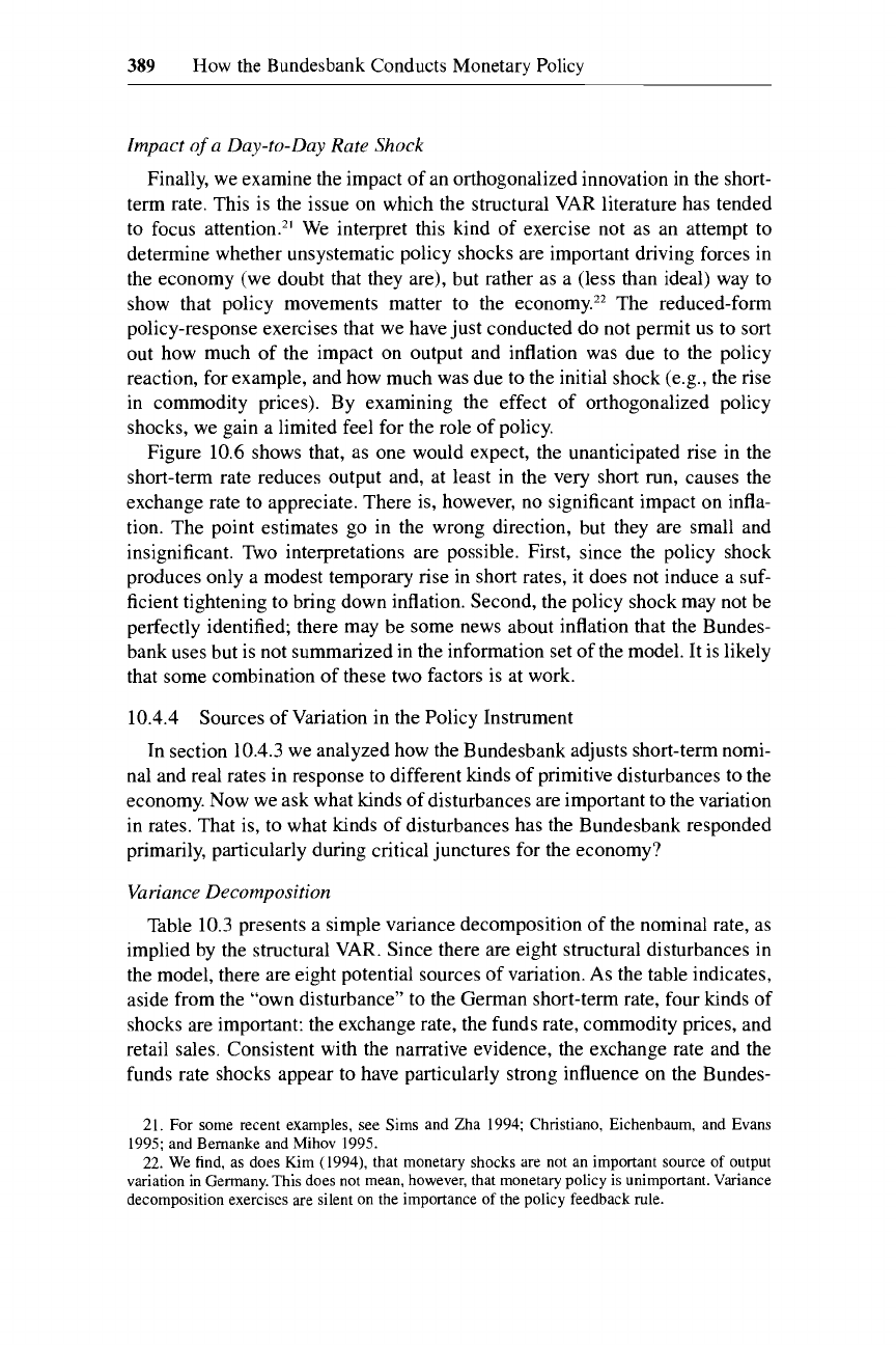
Finally, we examine the impact of an orthogonalized innovation in the short-
term rate. This is the issue
on
which the structural VAR literature has tended
to focus attention.z’ We interpret this kind of exercise not as an attempt to
determine whether unsystematic policy shocks are important driving forces in
the economy (we doubt that they are), but rather as a (less than ideal) way to
show that policy movements matter to the economy.22 The reduced-form
policy-response exercises that we have just conducted do not permit us to sort
out how much of the impact on output and inflation was due to the policy
reaction, for example, and how much was due to the initial shock (e.g., the rise
in commodity prices). By examining the effect
of
orthogonalized policy
shocks, we gain a limited feel for the role of policy.
Figure
10.6
shows that, as one would expect, the unanticipated rise in the
short-term rate reduces output and, at least in the very short
run,
causes the
exchange rate to appreciate. There is, however, no significant impact on infla-
tion. The point estimates go in the wrong direction, but they
are
small and
insignificant. Two interpretations are possible. First, since the policy shock
produces only a modest temporary rise in short rates, it does not induce a suf-
ficient tightening to bring down inflation. Second, the policy shock may not be
perfectly identified; there may be some news about inflation that the Bundes-
bank uses but is not summarized in the information set of the model. It is likely
that some combination of these two factors is at work.
10.4.4
Sources of Variation in the Policy Instrument
In
section
10.4.3
we analyzed how the Bundesbank adjusts short-term nomi-
nal and real rates in response to different kinds of primitive disturbances
to
the
economy. Now we ask what kinds of disturbances are important to the variation
in rates. That is, to what hnds of disturbances has the Bundesbank responded
primarily, particularly during critical junctures for the economy?
Variance Decomposition
Table
10.3
presents a simple variance decomposition of the nominal rate, as
implied by the structural VAR. Since there
are
eight structural disturbances in
the model, there are eight potential sources of variation. As the table indicates,
aside from the “own disturbance” to the German short-term rate, four kinds of
shocks are important: the exchange rate, the funds rate, commodity prices, and
retail sales. Consistent with the narrative evidence, the exchange rate and the
funds rate shocks appear to have particularly strong influence on the Bundes-
21.
For
some recent examples, see Sims and Zha 1994; Christiano, Eichenbaum, and Evans
1995; and Bernanke and Mihov 1995.
22.
We find, as does Kim (1994), that monetary shocks are
not
an important source
of
output
variation in Germany. This does
not
mean, however, that monetary policy is unimportant. Variance
decomposition exercises are silent
on
the importance
of
the policy feedback rule.

390
Richard Clarida and Mark
Gertler
Table
10.3
Variance Decomposition
for
the Nominal Interest Rate
Fraction
of
Forecast
Error
Variance
due
to
Horizon
(months)
e'p
e'p
e"'
el'
&
e" e" epr
6
0.01
0.04
0.03
0.01
0.16
0.01
0.57
0.16
12
0.06
0.03
0.08
0.01
0.15
0.01
0.50
0.17
24
0.11
0.02
0.18
0.01
0.13
0.01 0.42
0.13
48
0.12
0.02
0.22
0.01
0.13 0.01
0.38
0.12
bank behavior in the short run, together accounting for about
a
third of the
overall variation in the short-term rate over
a
six-month horizon. At twelve-
and twenty-four-month horizons, the commodity and retail sales shocks rise in
relative importance. Overall, the four shocks account for about half the varia-
tion in the short-term rate over twelve months and about
60%
over twenty-
four months.
Historical Decomposition
How do the four shocks account for the observed temporal pattern of Ger-
man short-term rates? Figure 10.7 presents a historical decomposition
of
the
variation in the nominal rate. The top panel shows the cumulative error in the
forecast of the nominal rate as the sample period unwinds. This measure indi-
cates how the short-term rate adjusted over time to shocks taking place during
the sample. The two periods of unforecastable declines in the short-term rate
are
the late 1970s and the late 1980s. These correspond to the periods of policy
easing cited in the narrative evidence. Similarly, the two periods
are
unfore-
castable increases are the early 1980s and the early 1990s, periods where the
informal evidence suggests policy tightness.
In the panels below we plot the contribution to the cumulative forecast error
by each of the four main sources (other than the own disturbance) of variation
in the short-term rate. Again, there is
a
reasonable correspondence between the
narrative and statistical evidence. Unexpected appreciations of the mark help
account for the unexpected rates declines in 1978-79 and 1986-87. The rise
in rates in the early 1980s is associated with
a
rise in real commodity prices, a
depreciation of the currency, and a rise in the funds rate, much as the narrative
evidence suggests. In particular these three factors appear to account for about
two-thirds of the rate increase that occurred at this time.
Finally, there are some direct signs that the real economy influences Bundes-
bank behavior. Unexpected declines in retail sales, along with an unexpected
appreciation of the mark, contributed to the decline in rates during the mid- to
late 1980s. Conversely, following this period, interest rates surged in large part
as a consequence of an unexpected sharp rise in retail sales, in conjunction
with an unexpected currency depreciation.
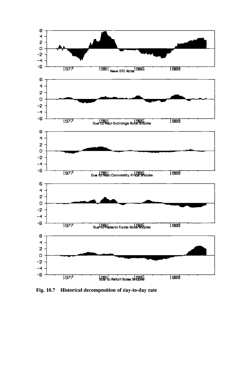
-
z-
-0
-z
I
19
I
’9
c-
z-
0
z
c
9

392
Richard Clarida and Mark
Gertler
10.5
Adding Structure:
A
Policy Reaction Function Based
on
Inflation
and Output Objectives
From the structural VAR we are able to ascertain how different primitive
disturbances to the economy influence the Bundesbank’s choice for the time
path of short-term interest rates. However, the policy reaction function we ob-
tain from this exercise-the identified VAR equation for the day-to-day inter-
est rate-is difficult to compactly summarize. We learn, for example, how the
Bundesbank has responded to movements in the D-mark. But we do not di-
rectly learn why. Was inflation the primary consideration?
Or
was concern
about output also a factor?
In
this section we estimate a compact and intuitive reaction function for the
day-to-day rate. We do
so
by imposing additional structure
on
the reaction
function obtained from the identified VAR. We assume that the Bundesbank
cares about stabilizing both inflation and output.
In
addition we allow for the
possibility that the Bundesbank is forward-looking in the sense that it adjusts
policy in response to anticipation of future inflation as opposed to simply past
inflation. Further, we take into account that in setting interest rates the Bundes-
bank may not know the current values of inflation and output (which is consis-
tent with what we assumed in section
10.4).
To form beliefs about expected inflation and output relative to their respec-
tive targets, the Bundesbank (we assume) filters the current and lagged infor-
mation about the economy, as captured by our eight variable VARs. Thus, for
example, we allow for movements in exchange rates to influence the day-to-
day rate, as the reduced-form evidence suggests. But we restrict these move-
ments to enter the policy reaction function based
on
the information they con-
tain about expected inflation and output (relative to capacity).
In
the end we
obtain a simple policy reaction function that relates the movement in short-
term rates to two “gap” variables that reflect the position of inflation and out-
put. As we show, this reaction function provides a very useful yardstick to
interpret the course of Bundesbank monetary policy.
10.5.1
Let
rs,
be the nominal day-to-day rate and
rsr
be the Bundesbank’s target for
this rate. Let
rrs,
denote the real day-to-day rate. Let
IT:-,
be the rate of inflation
from period
r
-
j
to
t
-
j
+
k:
equivalently,
IT-,
=
P,-,+~
-
p,-,,
where, as
before,
p,
is the logarithm of the price level. Also, as before,
ip,
is the logarithm
of output. Finally, let an asterisk denote the steady-state trend value of a vari-
able. We assume that the following two equations characterize the day-to-day
rate reaction function:
A Day-to-Day Rate Reaction Function
(5)
rsp
=
E,(+,}
+
rrs*
+
r”[E,(nf_,}
-
T*~]
+
y’p[E,{ip,
-
ip,*}]
and

393
How
the Bundesbank Conducts Monetary
Policy
rs,
=
Xrse
+
(1
-
~)[iw~rS,_,]
+
E,,
,=I
(6)
with
Cf;,,w,
=
1
and where the expectation operator
E,(
}
is conditioned on
the central bank’s information set at
t.23
As we noted in section
10.4,
the Bunde-
sbank observes certain variables, such
as
industrial production and consumer
prices, with a one-month lag.
Equation
5
is
a
slight variation of the type of reaction function that Taylor
(1993)
used to characterize the behavior of the Federal Reserve Board under
Alan Green~pan.~~ Underlying the rule is the notion that monetary policy is
neutral in the long run: the central bank cannot influence the long-run equilib-
rium values either of the real interest rate,
rrs*,
or of output,
@,*.
Due to nominal
rigidities, however, the central bank does have leverage over the short-term real
interest rate, and can thus influence the course of real activity in the short run.
The feedback rule has
a
general kind of lean-against-the-wind form.
Roughly speaking, it has the central bank raise the short-term real interest rate
as
either inflation or output rise relative to long-run trend. Trend inflation is the
steady-state inflation rate that the central bank is willing to accept, as
is
im-
plicit in its policy rule. That is, it is the rate of inflation that the central bank is
willing to accommodate when output is at its trend capacity value. It is thus
a
choice variable for the central bank. Trend output is the value of output that
would arise if the economy were currently in long-run equilibrium, and is thus
beyond the control
of
the central bank.
We assume further, according to equation
6,
that each month the Bundes-
bank sets the actual day-to-day rate equal to
a
convex combination of the target
rate and a weighted average of lagged rates. We allow for partial adjustment
because institutional factors in policymaking likely preclude the Bundesbank
from always reaching its target at the same frequency
of
our data. For example,
the effective decision-making interval may be longer than the monthly interval
we use. In practice we find that the adjustment period is usually very fast
(as
we show later).
An important difference between our specification and Taylor’s is that we
allow for the possibility that the central bank is forward-looking in its concern
for inflation, whereas Taylor instead assumes that the central bank responds to
inflation over the past year. In particular we consider three formulations of the
inflation gap variable: two that are forward-looking and one that corresponds
to Taylor.
Case
1
(forward-looking, one-year horizon):
23. We assume further that the Bundesbank responds only to movements in anticipated inflation
that are exogenous with respect to movements in the current short-term rate.
In
the estimation we
take account of this assumption explicitly by
using
instrumental variables.
For
this reason
our
rule
is not subject to the instrument instability problem discussed in Woodford (1994).
In
addition we
allow
for
partial adjustment
of
the interest rate, which is also a stabilizing factor.
24.
Taylor does not formally estimate his model. He does demonstrate, however, that his infor-
mal method
of
choosing parameters seems to
work
quite well for the Greenspan period.

394
Richard Clarida and Mark
Gertler
Case
2
(forward-looking, infinite horizon):
E,{T~-,)
-
T*~
=
limE,(T:}
-
T*~
=
E,{p,*
-
p,}
Case
3
(backward-looking, Taylor):
Case
1
is the mirror image of the Taylor specification: the central bank looks
one year forward at inflation, as opposed to one year back. Because the one-
year horizon is somewhat arbitrary, in case
2
we have the central bank respond
to expected total cumulative excess inflation. We define the latter as the ex-
pected percentage of change in the price level relative to trend indefinitely into
the future. This measure corresponds exactly to the percentage of difference
between the current trend and spot price levels. Intuitively, if the price level is
5%
below trend (i.e.,
p,*
-
p,
=
5%),
then the spot price level is expected to
grow
5%
faster than trend before reverting to long-run eq~ilibrium.~~
Finally,
for
comparison purposes, in case
3
we consider the backward-
looking measure that Taylor used. The expectation operator appears in this
case only because we allow for the possibility that the central bank may not
observe the current price level. (In equation
5
we similarly allow for the possi-
bility that it does not observe current output.)
We proceed by first computing the long-run equilibrium variables and the
gap variables that enter the policy reaction function. We use our estimated
structural VAR to obtain values
of
these variables for each calendar month. In
addition to obtaining inputs for the reaction function, we also extract informa-
tion that
is
helpful for judging the position of the economy and monetary pol-
icy, as we discuss below.
10.5.2
Long-Run Equilibria and Short-Run Deviations: A Historical
Decomposition of the Data
To identify the long-run equilibrium and the inflation and output gap vari-
ables, we return to the eight variable VARs of the German economy. We obtain
the steady-state value for any (stationary) variable in the VAR simply by find-
ing the k-step-ahead forecast of the respective variable, for
k
large.
Long-Run Equilibrium Interest Rates
and
Inpation
Figure
10.8
reports estimates of the long-run equilibrium values
of
the nom-
inal interest rate, inflation, and the real interest rate. In each panel is the time
25.
We
emphasize that stabilizing the gap
p:
-
p,
does not correspond to stabilizing the price
level around a deterministic trend. The empirical model
of
section
10.4
on
which we base the
analysis presumes a stochastic trend rather than a deterministic trend
for
the price level, owing to
the
presence
of
a unit root in the price level. The unit-root assumption (which is consistent with
the data) reflects the fact that the Bundesbank accommodates changes in the price level, as the
narrative evidence suggests (see section 10.3).

395
How
the
Bundesbank
Conducts Monetary Policy
15.0
12.5
10.0
7.5
5.0
2.5
-2.5
1
-5.0
0.0
Y
-7.5
'
79 83
a7
91
hflotlon
vn
Lnng
Run
Equlllbi-luni
75
15.0
12.5
-
10.0
-
-7.5
75
Ex
hts Re&ei-wHt Rots
v%ng
Run
Equlllb8~m
91
Fig.
10.8
Interest rates and inflation
series
of
the current value of the respective variable.
To
construct a time series
for the real interest rate, we used the observed nominal rate minus the inflation
forecast generated by the
VAR.
We computed steady-state values
of
6.28
for
the nominal rate,
3.2
for
inflation, and
3.1
for the real rate (simply the differ-
ence between the two). In each instance
the
estimates are close to the sample
mean (and are quite sensible).
As
we emphasized earlier, the steady-state inflation rate provides a measure
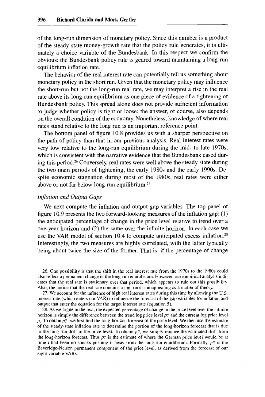
396
Richard Clarida and Mark Gertler
of
the long-run dimension of monetary policy. Since this number is
a
product
of
the
steady-state money-growth rate that the policy rule generates, it is ulti-
mately a choice variable of the Bundesbank. In this respect we confirm the
obvious: the Bundesbank policy rule is geared toward maintaining
a
long-run
equilibrium inflation rate.
The behavior of the real interest rate can potentially tell
us
something about
monetary policy in the short run. Given that the monetary policy may influence
the short-run but not the long-run real rate, we may interpret a rise in the real
rate above its long-run equilibrium
as
one piece of evidence
of
a
tightening
of
Bundesbank policy. This spread alone does not provide sufficient information
to judge whether policy is tight or loose; the answer,
of
course, also depends
on the overall condition
of
the economy. Nonetheless, knowledge of where real
rates stand relative to the long run is an important reference point.
The bottom panel of figure
10.8
provides us with
a
sharper perspective on
the path of policy than that in our previous analysis, Real interest rates were
very low relative to the long-run equilibrium during the mid- to late
1970s,
which is consistent with the narrative evidence that the Bundesbank eased dur-
ing this period.26 Conversely, real rates were well above the steady state during
the two main periods of tightening, the early
1980s
and the early
1990s.
De-
spite economic stagnation during most of the
1980s,
real rates were either
above
or
not far below long-run equilibrium.*’
Inflation and Output Gaps
We next compute the inflation and output gap variables. The top panel of
figure
10.9
presents the two forward-looking measures of the inflation gap:
(1)
the anticipated percentage
of
change in the price level relative to trend over
a
one-year horizon and
(2)
the same over the infinite horizon.
In
each case we
use the
VAR
model
of
section
10.4
to compute anticipated excess inflation.28
Interestingly, the two measures are highly correlated, with the latter typically
being about twice the size
of
the former. That is, if the percentage of change
26.
One
possibility is that the shift in the real interest rate from the
1970s
to the
1980s
could
also reflect a permanent change in the long-run equilibrium. However, our empirical analysis indi-
cates that the real rate is stationary over that period, which appears to rule out this possibility.
Also,
the notion that the real rate contains a unit root is unappealing as a matter of theory.
27.
We
account for the influence of high real interest rates during this time by allowing the
U.S.
interest rate (which enters our
VAR)
to influence the forecast of the gap variables for inflation and
output that enter the equation for the target interest rate (equation
5).
28.
As
we argue in the text, the expected percentage of change in the price level over the infinite
horizon is simply the difference between the trend log price level
p:
and the current
log
price level
p,.
To ohtainp:, we first find the long-horizon forecast of the price level. We then use the estimate
of the steady-state inflation rate
to
determine the portion of the long-horizon forecast that is due
to the long-run drift in the price level. To obtain
p:,
we simply remove the estimated drift from
the long-horizon forecast. Thus
p:
is the estimate of where the German price level would be at
time
t had been
no
shocks pushing it away from the long-run equilibrium. Formally,
p,*
is the
Beveridge-Nelson permanent component of the price level, as derived from the forecast of
our
eight variable
VARs.

397
How
the
Bundesbank Conducts Monetary Policy
7.5
I
-7.5
-
10.0
1
-
ptE&&-,
1
4'
s
87'
9
0'
' '
75'
'
78'
'
~flo~lo"'co2
10.0
7.5
5.0
2.5
0.0
-2.5
-5.0
-7.5
75'
E
78'
'
'8
1'
'
'8
4'
'
'
87'
'
'9
0'
' '
output
cop
-10,o
'
10.0
7.5
5.0
2.5
0.0
-2.5
-5.0
-7.5
-
10.0
Ex
Ante
Reol Intereet Rote
YB
Long
Run Equlllbrlum
Fig.
10.9
Inflation gaps, output gap, and real interest rates:
PI
GAP
12,
price-
level gap for one year;
PZ
GAP
240,
infinite horizon price-level gap
in the price level
is
expected to be
1%
above trend for the next year, then it is
likely to be a total of
2%
above trend over the indefinite future.
The middle panel
of
figure
10.9
presents our measure
of
the gap between
output and its long-run equilibrium,
ip,
-
ip,*.
To compute long-run equilibrium
output, we allow for the possibility that the trend drift in output is stochastic
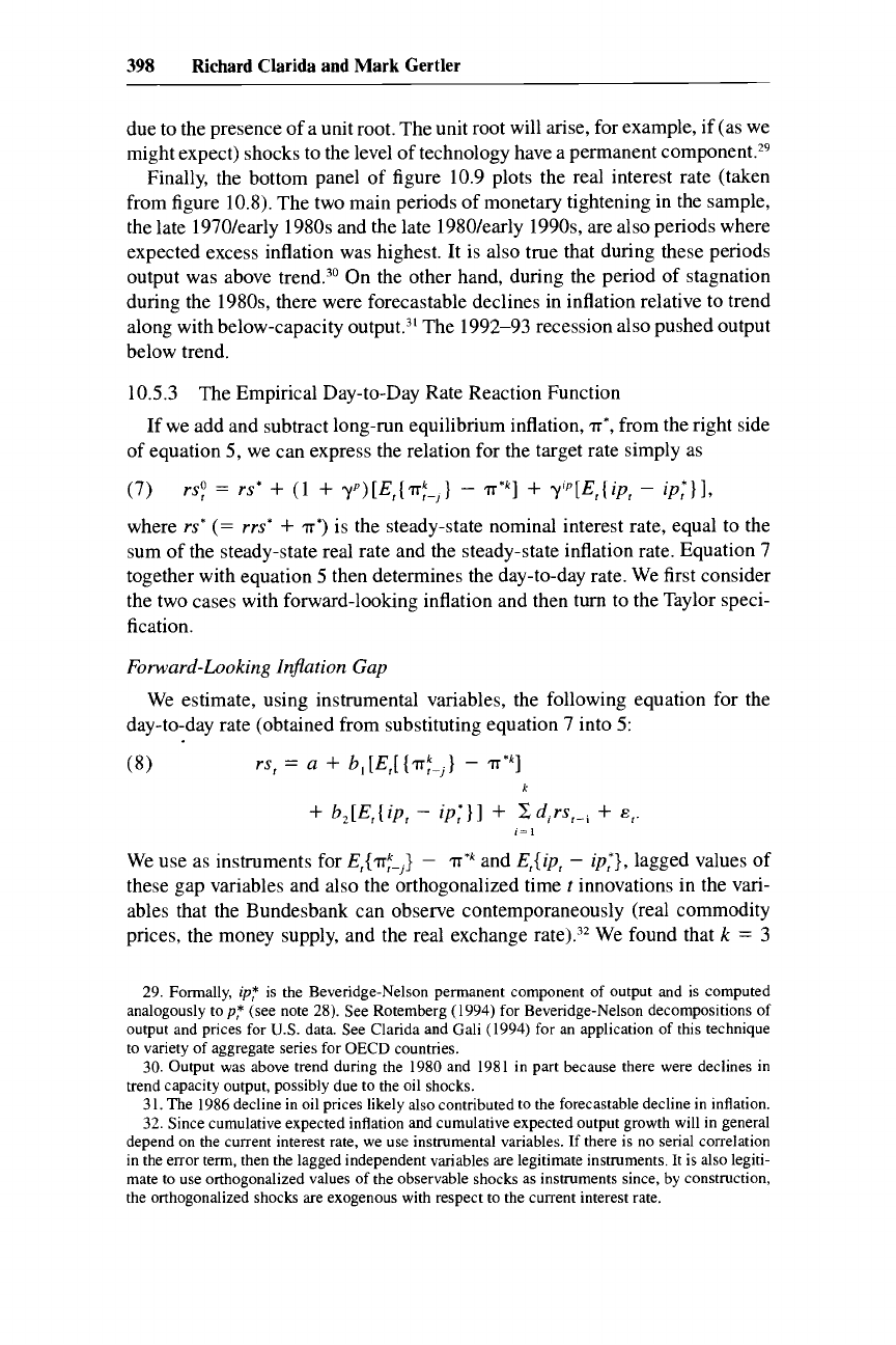
398
Richard Clarida and Mark Gertler
due to the presence of a unit root. The unit root will arise, for example,
if
(as we
might expect) shocks to the level
of
technology have a permanent component.29
Finally, the bottom panel of figure 10.9 plots the real interest rate (taken
from figure 10.8). The two main periods of monetary tightening in the sample,
the late 1970/early 1980s and the late 1980/early 1990s, are also periods where
expected excess inflation was highest. It is also true that during these periods
output was above trend.3o On the other hand, during the period of stagnation
during the 1980s, there were forecastable declines in inflation relative to trend
along with below-capacity outp~t.~' The 1992-93 recession also pushed output
below trend.
10.5.3 The Empirical Day-to-Day Rate Reaction Function
of equation
5,
we can express the relation for the target rate simply as
(7)
rs:
=
rs*
+
(1
+
YP)[E,{TT-,}
-
IT'^]
+
yrP[E,{ip,
-
@,*)I,
where
rs*
(=
rrs*
+
IT*)
is the steady-state nominal interest rate, equal to the
sum
of
the steady-state real rate and the steady-state inflation rate. Equation 7
together with equation
5
then determines the day-to-day rate. We first consider
the two cases with forward-looking inflation and then turn to the Taylor speci-
fication.
If
we add and subtract long-run equilibrium inflation,
IT*,
from the right side
Forward-Looking Injation
Gap
day-to-day rate (obtained from substituting equation 7 into
5:
(8)
We estimate, using instrumental variables, the following equation for the
rs,
=
a
+
b,[E,[
{
IT-^}
-
IT*^]
k
+
b,[E,{
ip,
-
ip,*}]
+
2
dirs,-,
+
E,.
,=I
We use as instruments for
E,{IT:-,)
-
IT*^
and
E,{ip,
-
ip,*},
lagged values of
these gap variables and also the orthogonalized time
t
innovations
in
the vari-
ables that the Bundesbank can observe contemporaneously (real commodity
prices, the money supply, and the real exchange rate).32 We found that
k
=
3
29. Formally,
ip:
is the Beveridge-Nelson permanent component of output and is computed
analogously top: (see note 28). See Rotemberg (1994) for Beveridge-Nelson decompositions of
output and prices for
US.
data. See Clarida and Gali (1994) for an application of this technique
to variety of aggregate series for OECD countries.
30.
Output was above trend during the 1980 and 1981 in part because there were declines in
trend capacity output, possibly due to the oil shocks.
3
1.
The 1986 decline in oil prices likely also contributed to the forecastable decline in inflation.
32. Since cumulative expected inflation and cumulative expected output growth will in general
depend on the current interest rate, we use instrumental variables.
If
there is no serial correlation
in the error term, then the lagged independent variables are legitimate instruments. It is also legiti-
mate to
use
orthogonalized values of the observable shocks as instruments since, by construction,
the
orthogonalized shocks are exogenous with respect to the current interest rate.
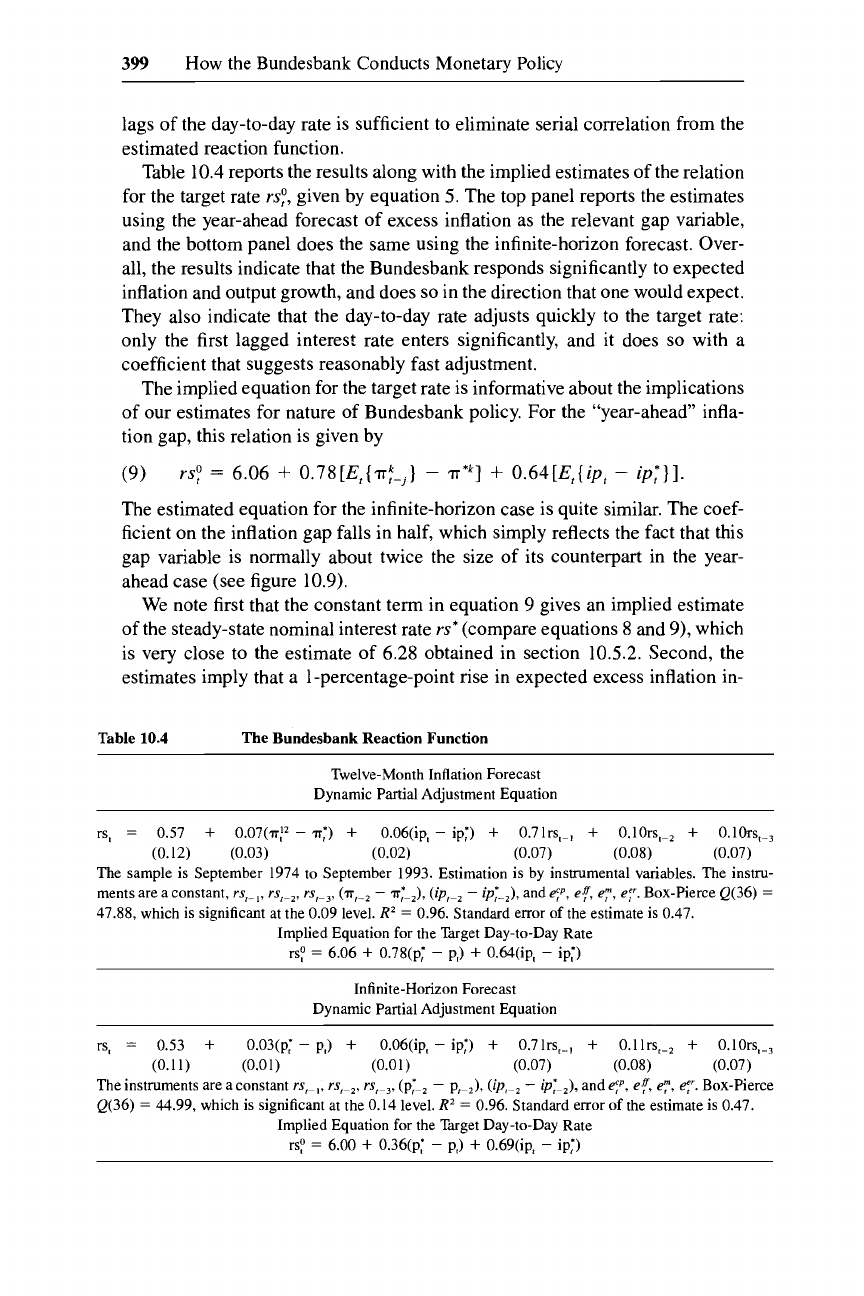
399
How the Bundesbank Conducts Monetary Policy
lags of the day-to-day rate is sufficient to eliminate serial correlation from the
estimated reaction function.
Table 10.4 reports the results along with the implied estimates of the relation
for the target rate
rsp,
given by equation
5.
The top panel reports the estimates
using the year-ahead forecast of excess inflation as the relevant gap variable,
and the bottom panel does the same using the infinite-horizon forecast. Over-
all, the results indicate that the Bundesbank responds significantly to expected
inflation and output growth, and does
so
in the direction that one would expect.
They also indicate that the day-to-day rate adjusts quickly to the target rate:
only the first lagged interest rate enters significantly, and it does so with a
coefficient that suggests reasonably fast adjustment.
The implied equation for the target rate is informative about the implications
of our estimates for nature of Bundesbank policy. For the “year-ahead” infla-
tion gap, this relation is given by
(9)
rsp
=
6.06
+
0.78[E,(~r-,]
-
~r*~]
+
0.64[Et{ip,
-
ipr]].
The estimated equation for the infinite-horizon case is quite similar. The coef-
ficient on the inflation gap falls in half, which simply reflects the fact that this
gap variable is normally about twice the size of its counterpart in the year-
ahead case (see figure
10.9).
We note first that the constant term in equation
9
gives an implied estimate
of the steady-state nominal interest rate
rs*
(compare equations 8 and
9),
which
is very close to the estimate of 6.28 obtained in section 10.5.2. Second, the
estimates imply that a 1-percentage-point rise in expected excess inflation in-
Table
10.4
The Bundesbank Reaction Function
Twelve-Month Inflation Forecast
Dynamic Partial Adjustment Equation
rs,
=
0.57
+
0.07(~r:~
-
P:)
+
O.O6(ip,
-
ip;)
+
0.71rs,-,
+
O.lOrs,-,
+
O.lOrs,-,
The sample is September 1974 to September 1993. Estimation is by instrumental variables. The instru-
ments are a constant,
rs,-l.
rs,-z,
rq3,
(T,-~
-
TT-J,
(i~,-~
-
@-J,
and
e;p.
ef,
e:.
el‘.
Box-Pierce Q(36)
=
47.88, which is significant at the 0.09 level.
R2
=
0.96. Standard error
of
the estimate is 0.47.
Implied Equation for the Target Day-to-Day Rate
rsp
=
6.06
+
0.78(p;
-
p,)
+
0.64(ip,
-
ip;)
(0.12) (0.03)
(0.02)
(0.07)
(0.08)
(0.07)
Infinite-Horizon Forecast
Dynamic Partial Adjustment Equation
rs,
=
0.53
+
O.O3(p;
-
p,)
+
O.O6(ip,
-
ip:)
+
0.71rs,_,
+
0.11rst-2
+
O.lOrs,_,
(0.11) (0.01) (0.01) (0.07)
(0.08)
(0.07)
The instruments are a constant
rs,-,,
rs,-2, rs,-g,
(pC2
-
P,-~),
(ipr-z
-
ip:-J,
and
e$,
ef,
ey,
q.
Box-Pierce
Q(36)
=
44.99, which is significant at the 0.14 level.
RZ
=
0.96. Standard error
of
the estimate is 0.47.
Implied Equation for the Target Day-to-Day Rate
rsp
=
6.00
+
0.36(pt*
-
p,)
+
0.69(ip,
-
ip;)

400
Richard Clarida and Mark
Gertler
Table
10.5
The Bundesbank Reaction Function, Asymmetric Response
to
Expected
Inflation and Disinflation
~
~-
-
~
Twelve-Month Inflation Forecast
Dynamic Partial Adjustment Equations
When
(a;?
-
a;'?)
>
0
rs,
=
0.53
+
0.15(~:~
-
a;'>)
+
O.OS(ip,
-
ip;)
+
0.71rs,-,
+
O.lOrs,-?
+
0.09rs,-,
When
-
a;")
<
0
rs,
=
0.53
+
0.03(7~:~
-
+
O.O6(ip,
-
ip:)
+
0.71rs,_,
+
0.10rs,_2
+
O.O9rs,-,
The sample is September 1974 to September 1993. Estimation is by instrument variables. The instruments
are aconstant,
rs,.i.
rs,-L.
rs,~.,,
(a,->
-
(ip,->
-
ip;-?),
ande;'',
e-f!
e;,
e?.
Box-Pierce Q(36)
=
54.64,
which is significant at the
0.03
level.
R2
=
0.96. Standard error of the estimate
is
0.47.
(0.13)
(0.08) (0.02)
(0.07)
(0.08)
(0.07)
(0.13)
(0.06)
(0.02) (0.07)
(0.08)
(0.07)
Implied Equations
for
the Target Day-to-Day Rate
rsy
=
5.6
+
1.60(~!~
-
a;'*)
+
0.56(ip,
-
ip:)
rs:
=
5.6
+
0.28(a!*
-
a:'2)
+
0.56(ip,
-
ip;)
When
-
a;")
>
0
When
(a;?
-
<
0
duces the Bundesbank to raise the target day-to-day rate by
78
basis points,
while a I-percentage-point increase in the output gap induces it to raise the
day-to-day rate
64
basis points.jj Thus, the Bundesbank does appear
to
condi-
tion policy on the state of the real economy, as our earlier analysis suggests.
One surprising feature of equation
9
is the implication that the Bundesbank
raises the target rate by less than the increase in expected inflation. One possi-
bility is that the policy rule is asymmetric with respect to inflation. That is, it
may be the case that if output is at capacity, the Bundesbank does not ease
much when expected inflation is below trend, but it tightens aggressively when
expected inflation is above trend. In this case the low coefficient on the infla-
tion gap could be due to the asymmetric policy response. We reestimated the
feedback rule to allow the response to differ across positive and negative infla-
tion gaps. The results support the asymmetry hypothesis.
Table
10.5
presents estimates of the asymmetric policy rule using the year-
ahead measure of excess inflation. Results for the infinite-horizon case are very
similar. Note that the response of the day-to-day rate to expected excess infla-
tion is positive and significant when the gap is positive, while it is not signifi-
cant when the gap is negative. The implied relation for the day-to-day rate is
5.60
+
1.60[E,{~f-,}
-
T*&]
+
0.56[E,(ip,
-
ip:)],
if
E,($
,}
-
7~*~
2
0.
5.60
+
0.28[E,(~:-,]
-
T*']
+
0.56[E,(ip,
-
ip,*)],
if
E,{T:-,]
-
T*~
<
0.
(10)
rs:
=
33. Each of the gap variables is multiplied by
one
hundred, implying that the respective coeffi-
cients are in basis points.

401
How
the Bundesbank Conducts Monetary Policy
When the inflation gap is positive, the Bundesbank raises the day-to-day rate
160 basis points in response to a 1% rise in expected excess inflation, implying
a real rate increase of 60 basis. On the other hand, it barely responds when
the inflation gap is negative. Allowing for an asymmetric policy response thus
appears to resolve the puzzle. Another interesting feature of equation 10 is that,
for the case of positive excess inflation, the estimated coefficients
on
the gap
variables are very close to the ones Taylor Thus, after allowing for our
modifications, it is not an exaggeration to suggest that the Bundesbank policy
rule during the post-Bretton Woods era bears a reasonable proximity to
the rule that Taylor employs to characterize U.S. monetary policy under
Greenspan.
As an informal way to judge both the fit and the implications of our esti-
mated reaction function, figure
10.10
plots the estimated target day-to-day rate
rsy
against the actual rate
rs,
for the linear policy rule described by equation 9.
Figure 10.11 does the same for the asymmetric rule described by equation 10.
In each case the target rate tracks the actual rate reasonably well, suggesting
that the model provides a decent accounting
of
Bundesbank policy.
It is interesting to note that, during the mid- to late 1970s, policy was some-
what easier than the norm for the era predicted by the model, which is consis-
tent with the narrative evidence. Specifically, the target rate was systematically
above the actual rate over this period. Conversely, policy was somewhat tighter
than the norm for the latter half of the sample. Particular episodes of relative
tightness were late 1982 to early 1983, when the real economy was still experi-
encing the effects
of
a severe recession, and 1992-93,
the
approximate time of
the breakup of the
EMS.
The relatively large gap between the actual and target
rates during this latter period provides support for the view that the Bundes-
bank was being unusually tough prior to the
EMS
collapse.
Interestingly, the linear model portrayed in figure
10.10
suggests that policy
was somewhat tougher than the norm during the mid-l980s, when the real
economy was stagnating and inflation was low. As figure 10.11 suggests, how-
ever, this discrepancy may be due to the failure to allow for an asymmetric
policy response during this period of below-trend inflation. The nonlinear
model, in contrast, tracks this period reasonably well.
The
Taylor
Spec$cation
We now reestimate the model using the difference between inflation over
the past year and trend inflation as the relevant gap variable. We try two varia-
tions. The first follows Taylor The second allows for partial ad-
justment.
34.
The corresponding coefficients
for
Taylor’s
rule are
1.5
on the inflation gap and
0.5
on the
output gap.
35.
Because Taylor used quarterly data, we measure the output gap using the quarterly average
of
our
monthly data.
We
also followed Taylor by assuming a deterministic trend
for
output.
The
results
are
not particularly sensitive to the method of detrending output, though allowing
for
a
stochastic trend does seem
to
improve the
fit.

\,
0.0
'
IIIIIIIII
IIIIIIIIII
Fig.
10.11
Asymmetric response
of
day-to-day interest rates to inflation, target
versus actual
Note:
See
equation
10.

403
How
the Bundesbank Conducts Monetary Policy
Table
10.6
Bundesbank Reaction Function: Taylor
Rule
Specification
Taylor Rule
rs:
=
6.35
+
0.71(~,
-
n:)
+
0.20(ip,
-
ip7,)
The sample is September 1974 to September 1993. Estimation is by
OLS.
Box-Pierce Q(36)
=
2,551.88,
which is significant at the
0.00001
level.
R2
=
0.43. Standard error of the estimate is
1.82.
ZPT,
is the
estimated trend in industrial production.
(0.12)
(0.07)
(0.03)
Taylor Rule with Partial Adjustment
rs,
=
0.33
+
0.01(~,
-
P')
+
O.O4(ip,
-
ipT,)
+
0.80rs,-,
+
0.11rst-2
+
0.03rs,-,
The sample is September 1974 to September 1993. Estimation is by
OLS.
Box-Pierce Q(36)
=
50.03,
which is significant at the 0.06 level.
RZ
=
0.96. Standard error
of
the estimate
is
0.50.
P,
is average
inflation over previous twelve months.
P*
is sample average inflation.
ipn,
-
ip,
is deviation
of
deterministic trend
ip
from actual
ip
averaged over the previous three months.
Implied Equation for the Target Day-to-Day Rate
rsp
=
6.6
+
0.15(~,
-
P')
+
0.84(ip,
-
ipT,)
(0.12) (0.02)
(0.01)
(0.07) (0.09) (0.07)
Table
10.6
reports the results. The top panel presents estimates of the stan-
dard Taylor specification. The coefficients are of the right sign, though the
coefficient on the inflation gap is too low to have the real rate move in the
wrong direction. More significantly, there
is
strong evidence of residual serial
correlation, suggesting the possibility of omitted variable bias. The bottom
panel presents the estimates for the case of partial adjustment. Including the
lagged day-to-day rate significantly reduces the residual correlation. On the
other hand, the coefficient on the inflation gap is no longer significant.
Finally, figure
10.12
plots the implied target rates for the two Taylor specifi-
cations against the actual day-to-day rate. The top panel portrays the case with
partial adjustment, while the bottom line portrays the standard specification.
Overall, the results suggest that the basic Taylor specification does not work as
well as our modified version.36
10.6
Concluding
Remarks
Despite the public focus on monetary targeting, in practice German mone-
tary policy involves the management of short-term interest rates, as it does in
the United States. The targets, however, do provide a reference point for deci-
sion making. The key feature is that they provide a benchmark policy rule that
is designed to meet a clearly articulated long-term inflation goal. While the
Bundesbank can and often does deviate from this rule, it must always provide
justification for doing
so.
By forcing this kind of focused discussion of Bunde-
sbank decisions, the targeting provides some discipline on the policy process.
36. We also try a variation that uses the coefficients that Taylor specified for
the
United States.
This specification does not improve
the
model's performance.
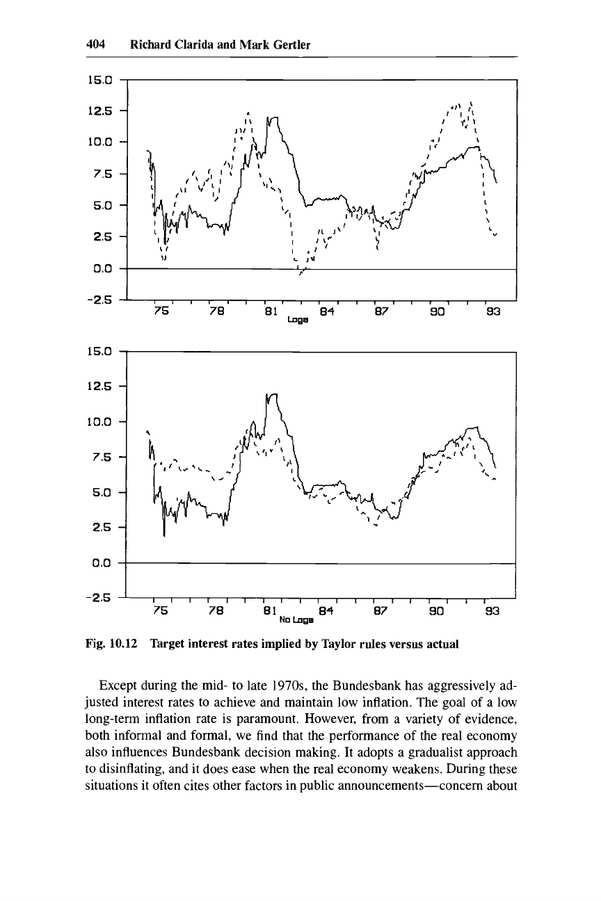
404
Richard Clarida and Mark Gertler
12.5
-
10.0
-
7.5
-
5.0
-
2.5
-
15.0
12.5
10.0
7.5
5.0
2.5
0.0
15.0
-2.5
O'O
I
75 78 81 84 87
so
93
No
Lnge
Fig.
10.12
Target interest rates implied by Taylor rules versus actual
Except during the mid- to late
1970s,
the Bundesbank has aggressively ad-
justed interest rates to achieve and maintain low inflation. The goal of a low
long-term inflation rate is paramount. However, from a variety of evidence,
both informal and formal, we find that the performance
of
the real economy
also influences Bundesbank decision making. It adopts a gradualist approach
to disinflating, and it does ease when the real economy weakens. During these
situations it often cites other factors in public announcements-concern about
405
How the Bundesbank Conducts Monetary Policy
maintaining the stability of exchange rate regimes, for example. Our results
suggest, however, that it is implicitly pursuing a countercyclical policy.
In
par-
ticular our formal analysis suggests that, for the most part, the Bundesbank has
adjusted short-term interest rates according to a kind of modified Taylor rule:
one that has the short-term rate adjust to anticipated inflation as opposed to
past inflation, and that allows for an asymmetric response of the short-term
rate to the inflation gap. In this respect there is a noteworthy parallel between
the conduct of Bundesbank policy in the post-Bretton Woods era and the oper-
ation of the Federal Reserve Board since
1987.
Despite obvious success in maintaining a low long-term inflation rate, the
Bundesbank has not been able to make disinflation a relatively painless pro-
cess,
as
the recessions of the early
1980s
and the early
1990s
suggest. Why it
has not reaped measurable gains from reputation building is a major puzzle,
one that a number of economists have noted.
As
we discussed earlier, the Bun-
desbank’s accommodation of inflation during the
1970s
may have influenced
public perceptions during
the
early
1980s,
though it is doubtful that this could
be the entire story. Further, since the Bundesbank aggressively pursued a low-
inflation policy over the
1980s,
this kind of explanation is less persuasive for
the most recent recession. On the other hand, it is possible that reunification
posed a special set of circumstances. Clearly, this general issue is an important
topic for future research.
We conclude with a perhaps mundane but nonetheless potentially important
lesson from the analysis.
A
current widely discussed issue is whether the mone-
tary policy should be aimed at achieving zero inflation. We learn from the
analysis that the Bundesbank has never tried to achieve exact price stability,
and has instead focused
on
a goal of
2%
long-run inflation. Concern about
measurement error in the price index-specifically, possible overstatement of
inflation due to imperfect adjustment for quality improvements-is the ratio-
nale provided for this objective. This measurement issue ought to be a key
concern of monetary policymakers, as it appears it is becoming in the United
States.
References
Ball, Laurence. 1994. What Determines the Sacrifice Ratio?
In
Monetary Policy,
ed.
N.
Bernanke, Ben, and Alan Blinder. 1992. The Federal Funds Rate and the Transmission
Bernanke, Ben, and Ilyan Mihov. 1995. Measuring Monetary Policy. Princeton Univer-
Bernanke, Ben, and Frederic Mishkin. 1992. Central Bank Behavior and the Strategy
Gregory Mankiw, 155-88. Chicago: University
of
Chicago Press.
of
Monetary Policy.
American Economic Review
82:901-21.
sity,
June. Mimeo.

406
Richard
Clarida
and
Mark
Gertler
of
Monetary Policy: Observations from Six Industrialized Countries. NBER Macroe-
conomics
Annual
7: 183-227.
Blanchard, Olivier J. 1989. A Traditional Interpretation of Economic Fluctuations.
American Economic Review 79: 1146-64.
Christiano, Lawrence J., Martin Eichenbaum, and Charles Evans. 1996. The Effects of
Monetary Policy Shocks: Evidence from the Flow
of
Funds. Review of Economics
and Statistics 78 (February): 16-34.
Clarida, Richard, and Jordi Gali. 1994. Sources of Real Exchange Rate Fluctuations:
How Important Are Nominal Shocks? Carnegie-Rochester Conference Series
on
Public Policy
41
(December): 1-56.
Deutsche Bundesbank. 1989. Policy Practices and Procedures. Frankfurt: Deutsche
Bundesbank.
Eichenbaum, Martin, and Charles Evans. 1995. Some Empirical Evidence on the Ef-
fects of Monetary Policy on Exchange Rates. Quarterly Journal of Economics 110
(November): 975-1
0
10.
Gali, Jordi. 1992. How Well Does the ISLM Model Fit Post-War U.S. Data? Quarterly
Journal
of
Economics
107
(May): 709-38.
Grilli, Vittorio, Donato Masciandaro, and Guido Tabellini. 199
1.
Central Bank Institu-
tions and Policies, Economic Policy.
Issing, Otmar. 1995. Stability of Monetary Policy, Stability of the Monetary System:
Experience with Monetary Targeting
in
Germany. Deutsche Bundesbank. Mimeo.
Kahn, George, and Kristina Jacobson. 1989. Lessons from West German Monetary Pol-
icy. Federal Reserve Bank of Kansas City Economic Review (April): 18-34.
Kim, Soyoung. 1994. Does Monetary Policy Matter in the G-6 Countries. Yale Univer-
sity. Mimeo.
Kim,
Soyoung, and Nouriel Roubini. 1995. Liquidity and Exchange Rates: A Structural
VAR Approach. New York University. Mimeo.
Kole, Linda, and Ellen Meade. 1994. Searching for the Holy Grail: An Examination of
German Money Demand after Unification. Federal Reserve Board. Mimeo.
Neumann, Manfred J. M., and Jurgen Von Hagen. 1993. Germany. In Monetav Policy
in Developed Countries, ed. Michele Fratianni and Dominick Salvatore. London:
Greenwood Press.
Rotemberg, Julio. 1994. Prices, Output, and Hours: An Empirical Analysis Based on
a
Sticky Price Model. Massachusetts Institute of Technology. Mimeo.
Sims, Christopher A,, and Tao Zha. 1994. Does Monetary Policy Generate Recessions?
Using Less Aggregate Price Data to Identify Monetary Policy. Yale University.
Mimeo.
Taylor, John. 1993. Discretion versus Policy Rules in Practice. Carnegie-Rochester
Conference Series
on
Public Policy 38 (December): 195-214.
Trehan, Bharat. 1988. The Practice of Monetary Targeting: A Case Study of the West
German Experience. Federal Reserve Bank
of
San Francisco Economic Review
(spring): 30-44.
Tsatsaronis, Konstantinos. 1993. Bank Lending and the Monetary Transmission Mecha-
nism: The Case of Germany. Mimeo.
Uctum, Merih. 1995. European Integration and Asymmetry in the EMS. Federal Re-
serve Bank of New York. Mimeo.
Von Hagen, Jurgen. 1994. Inflation and Monetary Targeting in Germany. University of
Mannheim and Indiana University. Mimeo.
Woodford, Michael. 1994. Nonstandard Indicators for Monetary Policy. In Monetary
Policy, ed. N. Gregory Mankiw, 95-1 15. Chicago: University
of
Chicago Press.
407
How
the Bundesbank Conducts Monetary
Policy
Comment
Rudiger Dornbusch
The paper by Clarida and Gertler (ClaGer for short) offers a revisionist view
of
the Bundesbank. The myth has been that of an institution fighting inflation,
with little other concern, predominantly with an M3-oriented strategy. ClaGer
make a good case that the Buba is no different from most other central banks,
notably the Fed. They establish a reaction function with inflation and output
gaps as the chief determinants of an interest rate-oriented policy. Amazingly,
M3
plays
absolutely
no role in the story.
That rendition is nothing short of dramatic. After all, the Buba keeps talking
about
M3
and keeps getting entangled in the huge discrepancies between tar-
geted
M3
and the large departures of actual
M3.
I
argue that ClaGer have done
a great job in bringing Buba policy down to earth, but that they have not gone
far enough. Whenever
M3
goes wild, the Buba is mired in its own rhetoric.
That is precisely when the Buba does
not
do the obvious, that is, cut rates in
the midst of a no-inflation, serious-downturn situation. The first half of 1996
is a case in point.
I
review briefly the Buba folklore, consider the ClaGer rendition, and move
on to an attempt to reestablish some role for
M3
in interpreting Buba policy
mistakes. The point is, when common sense and adherence to
M3
targets point
in opposite directions, the Buba sometimes goes the wrong way.
The Folklore
The setting is shown in figure
10C.l,
which reports German CPI inflation
(for twelve-month periods). Three major inflation episodes are apparent. Com-
ing out of the destructive experience of a hyperinflation, a monetary write-off
in 1948, dollar dependence under Bretton Woods, and an unsuccessful encoun-
ter with supply-shock inflation, the Buba places great weight on a firm anchor.
A premium is placed on a simple message that allows the Buba to tie its hands
against any temptation to pursue a long-run inflationary strategy.
M3
is thought to offer precisely that assurance.
The relationship in question derives from a stable long-run
M3
real money
demand. The velocity of
M3,
other than for a 1% per year downward trend, is
near-constant over the medium term. Accordingly, there is a relationship be-
tween the medium-term price level
P*,
the level of potential output
Y*,
trend
velocity
V*,
and the trend price level
P*:
(1)
P*
=
V*M3/Y*.
Such
a
relationship existed in the United States until Goodhart’s law caught up
with it; in Germany it is believed still to exist. Empirical evidence for various
Rudiger Dornbusch is the Ford Professor of Economics and International Management at the
Massachusetts Institute
of
Technology and
a
research associate
of
the National Bureau
of
Eco-
nomic Research.

408
Richard Clarida and Mark Gertler
-I
O.
1964 1968 1972 1976 1980 1984 1988
1992
1996
Fig.
10C.l
Germany:
CPI
inflation (percentage during the past twelve months)
OECD countries is reviewed in Hoeller and Poret
(1991).
In
the case of Ger-
many,
as
recently as
1995
the evidence
of
a
stable
M3
equation has been re-
viewed by the Buba
(Monthly
Report,
July
1995)
and the conclusion remains:
yes, there
is
a
stable demand for
M3,
and
as
a
consequence,
M3
targeting is
the basis
of
a sound monetary strategy. “Most of the empirical studies now
available show positive results. Hence German monetary policy makers can
continue to count on lastingly stable money demand’ (Deutsche Bundesbank
1995).
With a stable money-demand equation in hand, the Buba operates its policy
by setting annual
M3
growth corridors. The extraordinary claim of ClaGer is
that this is just camouflage.
A
plain vanilla reaction function
i
la Taylor ex-
plains what goes on,
M3
is just not there!
The Clarida-Gertler Rendition
The ClaGer paper reviews in careful detail the broad trends in Buba policy
and then comes down to the hard work of identifying just what goes on. The
central conclusion is that policy can be modeled as
a
reaction function. The
short-term interest rate is expressed
as
a
function of the discrepancy between
actual and long-run target inflation and the output gap. There is also a dynam-
ics to the rate setting, which
I
skip here. The real interest rate target level,
R,
that emerges
is
409
How
the Bundesbank Conducts Monetary Policy
where
r*
is the long-run real interest rate (3%), while
IT
and
IT*
are the
forward-looking inflation forecast and the long-run equilibrium rate. There are
important technical features in the modeling of the inflation deviation and the
output gap-they are forward-looking using estimates of a variable autoregres-
sion
(VAR)
model, but that is not a central issue here. The focus rather is on
the finding that inflation gaps and the output gap explain what the Buba does
with interest rates;
M3
is just not part of the story. (Not part of the story over
and above the role in the
VAR
forecast.) Figures 10.10 and 10.11 show the
target interest rate emerging from the reaction function as well as the actuals,
and it
is
clear that the model works surprisingly well.
The details of the coefficient deserve attention. ClaGer experiment with
asymmetries and their conclusion is this.
The Buba responds to a 100-basis-point inflation shock with a 60-basis-point
increase in real interest rates.
A
100-basis-point favorable inflation surprise induces only a 28-basis-point
cut in nominal interest rates or, equivalently, a 72-basis-point increase in real
rates. Thus interest rate policy does not fully accommodate disinflation.
A
100-basis-point increase in the output gap (measured by industrial produc-
tion) includes a 64-basis-point increase in nominal and real interest rates.
A
central question in this reaction-function setting
is
what the long-run
or
target level of inflation is. ClaGer find that the level of
IT*
is 3.2%. This is
surprising because, at least since the 1980s, the rhetoric is 0-2%. Even
so,
they
refer to their finding as “sensible” and note: “the steady-state inflation rate
provides a measure of the long-run dimension of monetary policy. Since
this
number is a product of the steady-state money-growth rate that the policy rule
generates, it is ultimately a choice variable of the Bundesbank.”
Bundesbankers would be surprised to find that their long-run strategy im-
plies a 3.2% inflation! The authors may have come to their unusual finding
because their sample period includes the supply-shock period of the 1970s,
where the Buba was taken by surprise and spent a long time with inflation rates
that were out of sight. That argues for using the post-oil shock sample period,
where the recognition is made explicitly that moderate inflation in long-run
averages requires that any overshooting be followed by periods of undershoot-
ing. This point is particularly obvious in the
1995-96
discussion rendered in
the
Monthly
Reports.
There we read that, yes, inflation is safely below
2%
but
that is not an invitation for expansion. It has to be kept low and pushed down
so
that the long-run averages come out right. Some of this may be brink-
manship, but the fact is that Germany is in a slump and the Buba is not rushing
out to give relief. In sum, modeling strategy around a target of 3.2% infla-
tion is plainly
a
misreading of what the Buba
is
about, at least in the last
decade.

410
Richard Clarida and Mark
Gertler
M3 Matters
A second question about
the
reaction functions is just how successful they
are.
I
note that, indeed, the major episodes of large rate changes are captured
well. But as figure
10.11,
for example, shows, there are major and persistent
discrepancies between target and actual rates. Thus, in
1978-81
targets exceed
actuals persistently, while in
1982-83
the converse is the case. Once again, in
1991-93
actuals exceed targets significantly. The figure shows that by
1993
the
target nominal rate would have been below
2.5%!
It is tempting to believe that
M3
has to do with precisely these persistent discrepancies between the
reaction-function prediction and the outcome. Consider, for example, the expe-
rience
of
the
1990s.
ClaGer show large discrepancies
of
target and actual rates
in
1993-93.
Table
10C.l
shows large overshooting of
M3
relative to target. Is
it not tempting to consider that the Buba gave some weight to the
M3
over-
shooting, and for that reason the reaction function, which does not contain
M3,
misfires?
It is tempting therefore to suggest a formulation well within the spirit of
ClaGer but with a Buba special. The real interest rate equation might be
stated as
(3)
R‘
=
y
R
+
(1
-
y)M3
Overshoot.
In this fashion we capture the factors ClaGer identify in the Taylor-style rendi-
tion of the reaction function but at the same time leave room for the situation
where
M3
overshooting puts the Buba in a bind.
An episode along these lines is surely the early
part
of
1996.
As figure
10C.2
shows, after a slow year
of M3
growth, far below target, in
1996 M3
growth
took off like a bat out of hell. The Buba is bewildered: the economy with low
inflation and no growth needs stimulus, but
M3
is running wild. What to do?
The Buba is all tied in knots, hoping that
M3
will slow down, the economy
will recover, and
M3
targeting can be kept alive.
European Monetary Union
Another direction to look, if we want to understand just how committed the
Buba is to monetary targeting, is the setup for Europe’s new monetary institu-
tions. As Europe moves toward a common money, the operating instructions
for the European Central Bank are being drafted. The Buba has weighed in
heavily: predictably, with monetary targeting. The Buba has denounced
inflation-targeting U.K.-style and has insisted on monetary-aggregates tar-
geting. Specifically, Buba president Tietmeyer
(1996)
argued that stability of
real money demand in Europe, outside Germany, was a fact: “As a result, a
monetary aggregate strategy, in my judgment, is the most convincing concept
for monetary policy in the monetary union. With its use, the European Central
Bank could inherit the reputation
of
the Bundesbank.
For
a young institution
such as ECB will be, this seems certainly attractive” (Tietmeyer
1996).
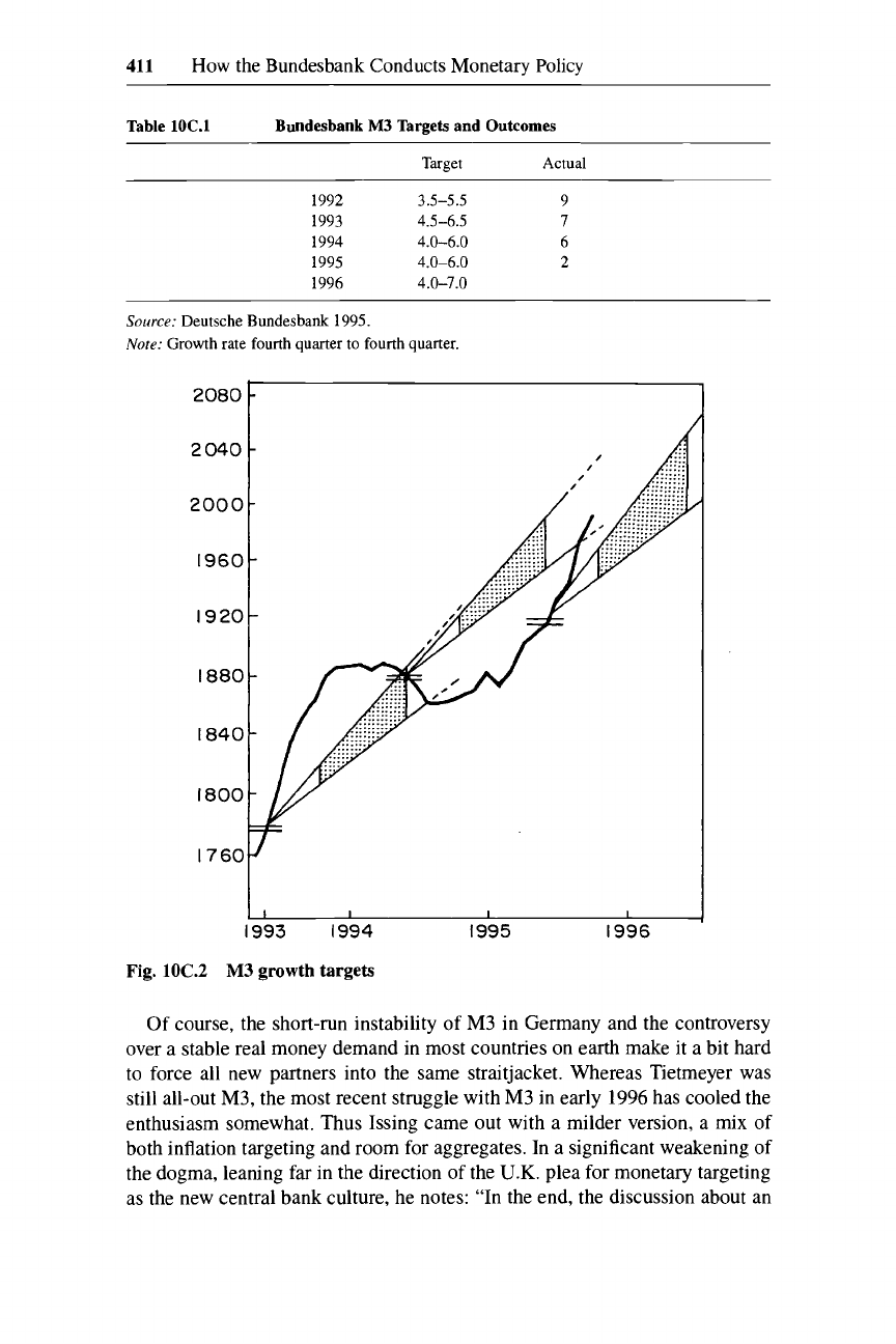
411
How
the Bundesbank Conducts Monetary Policy
Table
10C.l
Bundesbank
M3
Targets and Outcomes
Target Actual
1992 3.5-5.5 9
1993 4.5-6.5 7
1994 4.0-6.0 6
1995 4.0-6.0 2
1996 4.0-7.0
Source:
Deutsche Bundesbank
1995.
Nore:
Growth
rate
fourth
quarter
to fourth quarter.
2080
2
040
2000
I960
I920
I880
I840
I800
I760
I
1 1
1
1993 1994 1995
1996
Fig. 10C.2
M3
growth
targets
Of course, the short-run instability of
M3
in Germany and the controversy
over a stable real money demand in most countries on earth make it a bit hard
to force all new partners into the same straitjacket. Whereas Tietmeyer was
still all-out
M3,
the most recent struggle with
M3
in early
1996
has cooled the
enthusiasm somewhat. Thus Issing came out with a milder version,
a
mix of
both inflation targeting and room for aggregates. In a significant weakening of
the dogma, leaning far in
the
direction
of
the
U.K.
plea for monetary targeting
as the new central bank culture, he notes: “In the end, the discussion about an
412
Richard Clarida and
Mark
Gertler
optimal concept cannot be an Either-or but must rather
a
combination of mon-
etary aggregates strategy and inflation targeting” (1996,
8;
see
also
Konig
1996).
The point remains:
M3
has been there, is there, and is not about to disappear.
The German saving public
(die
Sparer)
have been brought up to trust in the
simple quantity theory, and they are not ready to believe in a new institution
and
new operating instructions
all
at once.
It is appropriate to end on a quote from the
Zuuberlehrling
of
Goethe: “Herr,
die Not is gross, die ich rief die Geister, werd ich nun nicht
10s.”
References
Deutsche Bundesbank. 1995.
Annual Report.
Frankfurt: Deutsche Bundesbank.
Hoeller,
P.,
and
P.
Poret. 1991.
Is
P*
a Good Indicator of Inflationary Pressures
in
OECD Countries?
OECD Economic Studies,
no.
17.7-30.
Issing, Otmar. 1996. Speech to the Bavarian Assembly.
Deutsch Bundesbank Auszuge
aus Presseartikeln,
no. 30, May
5,
1996,
8.
Konig, Reiner. 1996. The Bundesbank’s Experience in Monetary Targeting. In
Mone-
tary Policy Strategies in Europe,
ed. Deutsche Bundesbank. Munich: Verlag Wahlen.
Tietmeyer, Hans. 1996. Speech to the Colloquium on Globale Finanzmarkte und
EWWU, Goethe Universitat, Frankfurt.
Deutsche Bundesbank Auszuge aus Pressear-
tikeln,
no. 27, April
4,
1996,4.
